2.5.3. Alignment elements

2.5.3.1. Horizontal alignment elements

Internally a horizontal alignment is a chain of four primitive element types: Line, Arc, Clothoid spiral and Cubic parabola spiral. Each element exposes a common interface — start point, start direction, length, end point, end direction, point at distance, direction at distance, curvature at distance — and the chain accumulates them into a continuous, raw-distance parameterised centreline. The displayed station value is then RawToStation(raw) which applies the Start Station offset and any station equations defined on the geometry.

The sign convention used everywhere:

Curvature k = dψ/ds (rate of heading change with arc length). Left turn (counter-clockwise) ⇒ k > 0.
Offset: positive = right of travel, negative = left.
Bearing: the project’s angular units (degrees / gradians) measured from North, increasing clockwise — exactly as you would read on a total-station compass.

2.5.3.1.1. Line

The simplest segment — a straight line of length L = ‖(End − Start)‖ between two end-points with a constant direction ψ = ArcTan2(ΔY, ΔX).

Field	Description
Start X	Easting of the start point
Start Y	Northing of the start point
End X	Easting of the end point
End Y	Northing of the end point
Start Sta	Station value at the start point

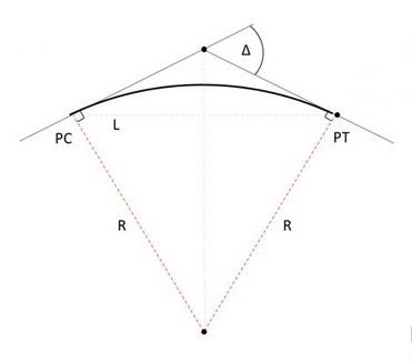
2.5.3.1.2. Arc (circular)

A circular arc of constant radius R, defined by a centre point (cx, cy), a starting direction and a length. The internal representation uses signed curvature so that the same data type covers both turn directions:

\[k(s) = \pm \frac{1}{|R|},\qquad \psi(s) = \psi_0 + k \cdot s,\qquad \bigl(x(s),\,y(s)\bigr) = \bigl(cx,\,cy\bigr) + R\!\bigl(\sin\psi(s),\,-\cos\psi(s)\bigr)\]

with k > 0 for a true left turn (CCW) and k < 0 for a right turn (CW). The Clockwise flag stored on each arc element drives the sweep direction at draw time.

Field	Description
Center X	Easting of the centre point
Center Y	Northing of the centre point
Bearing	Bearing of the start tangent (gradians)
Start Sta	Station value at the start point
Length	Arc length
Radius	Signed: `+` right turn, `−` left turn

Note

The legacy TCML / ALM <HElement> import format encodes the arc turn with a signed Radius attribute. Some exporters use the opposite sign convention; the current version derives turn direction from geometry (continuity with the previous element’s end direction) rather than the radius sign, so files from either convention round-trip correctly.

2.5.3.1.3. Clothoid spiral

A clothoid (Euler spiral, Cornu spiral) is the transition curve whose curvature varies linearly with arc length:

\[k(s) = \frac{1}{R(s)} = \frac{s}{A^{2}},\]

where A is the clothoid parameter. The signature property A² = R · L is exactly what makes the curve so useful in roads and railways: the transverse acceleration on a vehicle at speed v is v² · k(s), and a clothoid distributes the change of acceleration at a constant rate — there is no abrupt jerk where a tangent meets an arc. Highways and rail lines therefore use a clothoid between any tangent and circular curve (and again between that curve and the next tangent), to keep the lateral acceleration profile a continuous ramp.

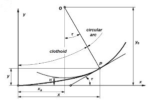
2.5.3.1.3.1. The intrinsic equations

Place the origin at the inflection point (where curvature is zero) and align the X axis with the local tangent. With K = R · L (the product radius × length of the spiral, also written R · L in the editor and in .alm files as RLValue), the position at a parametric distance D along the spiral is given by the Fresnel-integral series expansion (kept to the third term, which is more than enough for civil-engineering distances):

\[x = \frac{D^{3}}{6\,K} \;-\; \frac{D^{7}}{336\,K^{3}} \;+\; \frac{D^{11}}{42\,240\,K^{5}}\]

\[y = D \;-\; \frac{D^{5}}{40\,K^{2}} \;+\; \frac{D^{9}}{3\,456\,K^{4}}\]

The tangent direction at distance D is

\[\tau(D) = \frac{D^{2}}{2\,K},\]

so curvature grows linearly: k(D) = D / K = D / (R · L) — at D = L we have k = 1/R and the clothoid meets the circular arc tangentially without jerk.

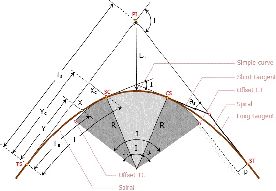
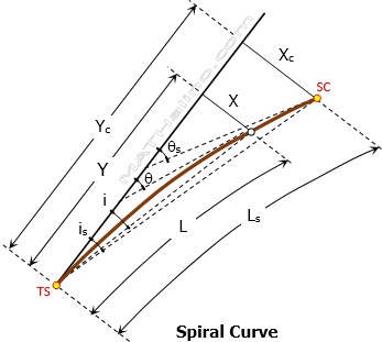
(The .gif versions of these figures in the source tree are animations that visualise how a vehicle’s lateral acceleration ramps up linearly along the spiral.)

In the editor a clothoid is described either by its start point / tangent / length / start radius / end radius, or by its origin point (the inflection point where curvature is zero) plus the same length and R·L value. Internally the engine always stores (start point, start direction, start radius, end radius, length, clockwise) and recomputes everything from that minimal description.

2.5.3.1.3.1.1. Defining a clothoid by start point

Field	Description
Start X	Easting of the start point
Start Y	Northing of the start point
Bearing	Tangent bearing at start (gradians)
Start Sta	Station value at the start point
Length	Arc length of the spiral
Start Radius	`+` right, `−` left (∞ for entry spiral)
End Radius	`+` right, `−` left (∞ for exit spiral)

2.5.3.1.3.1.2. Defining a clothoid by origin

Field	Description
Origin X	Easting of the inflection (zero curvature)
Origin Y	Northing of the inflection
Bearing	Tangent bearing at origin (gradians)
Sta at Origin	Station value at the origin
Length	Arc length of the spiral
R · L	Clothoid parameter (radius × length)
Start Sta	Station value at the start point

2.5.3.1.4. Cubic parabola spiral

The cubic parabola is the spiral classically used by the British, Indian and a number of Commonwealth railway standards as a simpler substitute for the clothoid. It tracks curvature linearly along the chord (rather than along the arc length, as the clothoid does), which produces a small but bounded discrepancy with the true spiral for the modest deflection angles typical in railway practice. For small deflections the two curves are visually indistinguishable.

The position is, in the same intrinsic frame as the clothoid:

\[y = \frac{x^{3}}{6\,K}, \qquad K = R\cdot L, \qquad \tau(x) \approx \frac{x^{2}}{2\,K}.\]

That is — directly a cubic in x, rather than the Fresnel-integral series the clothoid requires. The single relation y = x³/(6K) is the property that makes the cubic parabola attractive for slide-rule / table-based field setting-out; the curvature is

\[k(x) = \frac{y''}{\bigl(1 + y'^{2}\bigr)^{3/2}} = \frac{x / K}{\bigl(1 + x^{4}/(4K^{2})\bigr)^{3/2}},\]

which approaches x/K for small x²/K — i.e. for the angles encountered on a railway curve (≤ ~10°) the cubic parabola behaves as a clothoid to a few millimetres on a 1 km curve.

When to use which spiral:

Clothoid — modern roads, high-speed rail, all LandXML interchange. Continuous curvature growth = s/K exactly.
Cubic parabola — heritage railway alignments, certain UK / IR / Australian rail standards.

The cubic-parabola element accepts the same input modes as the clothoid (by start point or by origin); the engine fits the same (start, start direction, start radius, end radius, length, clockwise) internal representation, then evaluates points and tangents using the cubic relation above instead of the Fresnel series.

Field	Description
Start X	Easting of the start point
Start Y	Northing of the start point
Bearing	Tangent bearing at start (gradians)
Start Sta	Station value at the start point
Length	Length of the parabolic spiral
Start Radius	`+` right, `−` left
End Radius	`+` right, `−` left

Alternative: define by origin, R·L and length, same as the clothoid.

2.5.3.2. Vertical alignment elements

The vertical profile (chainage ➜ elevation) is built from two element families:

Grade: a straight segment of constant slope g = (h_end − h_start) / (sta_end − sta_start).
Vertical curve: a parabolic vertical curve (the highway convention) or a circular vertical curve (the railway convention). Both elements interpolate elevation between two grades; the editor and importers accept both.

2.5.3.2.1. Parabolic vertical curve

The parabolic VC is parameterised by the PVI (point of vertical intersection) and the curve length L. With incoming grade g₁ and outgoing grade g₂:

\[h(s) = h_{BVC} + g_{1}\,s + \frac{g_{2} - g_{1}}{2\,L}\,s^{2}\]

over s ∈ [0, L], with BVC = beginning of vertical curve (half the length back from the PVI). The convention R · 100 = L / (g₁ − g₂) defines an equivalent radius used in some import/export formats (+ convex / crest, − concave / sag).

2.5.3.2.2. Circular vertical curve

A circular VC is a true circular arc in the (station, elevation) plane. The engine accepts both forms on import; for typical highway geometries the two are visually indistinguishable for L ≪ R.

2.5.3.2.3. Profile editor fields

Grade element:

Field	Description
Start Height	Elevation at the start
Start Station	Chainage at the start
End Height	Elevation at the end
End Station	Chainage at the end

Vertical curve element:

Field	Description
Start Height	Elevation at the start (BVC)
Start Slope	Incoming grade (rise/run)
Start Station	Station at the BVC
Length	Curve length `L`
Radius	`+` crest (convex), `−` sag (concave)

2.5.3.3. Cross-section collections

Each of the following is a list of segments (startSta, startValue, endSta, endValue), linearly interpolated between the segment endpoints and held flat outside the defined range. The editor exposes them as separate grids and they round-trip in LandXML, ASCII and native .alm.

2.5.3.3.1. Horizontal offset alignment

Defines an offset centreline parallel to the geometric centreline. Setout(Chainage, Offset, Dh) with Mode = Offset Axis measures the offset from this offset centreline instead of the geometric centreline.

Field	Description
Start Station	Start chainage
Horizontal Off	Lateral offset value
End Station	End chainage
Horizontal Off	Lateral offset value

2.5.3.3.2. Vertical offset alignment

Adds a vertical offset to the profile elevation.

2.5.3.3.3. Superelevation left / right

Cross-fall of the road surface left / right of centreline, expressed as a percentage of % (positive = outer edge higher). The setout engine multiplies this with the offset to compute point height above the alignment elevation.

2.5.3.3.4. Superelevation-offset left / right

Per-station offset to add to the superelevation values (rarely used; provided for full LandXML compatibility).

2.5.3.3.5. Widening left / right

Per-station lateral widening of the road edge (positive widens outward). The editor optionally draws the widened edges on the horizontal plan.

2.5.3.3.6. Cant (rail only)

The rail-bank value (cm) per chainage, used by Mode = Rail setout. The cant is independent of the road super-elevation collections; it represents the height difference between the two rails on a track centreline. See Rail alignment — cant, CTC and UTC for the detailed CTC/UTC geometry that converts (CTC offset, CTC Dh, cant, gauge, rotation point) into the world (X, Y, Z, Theta).