2.6.5. Greek Projections Calculator

2.6.5.1. Overview

The Greek Projections calculator turns raw total-station measurements into precise grid coordinates in the Greek reference systems. For each pointing (horizontal angle, zenith angle, slope distance) taken from a known station to a target, it applies the full chain of projection corrections — height difference with curvature and refraction, reduction to sea level, chord and arc reductions, the grid line-scale factor, and the arc-to-chord (t−T) angle correction — and returns the target’s X, Y, H.

It is a modern port of the legacy IQSoft Provolika tool and reproduces its results faithfully. Supported projections:

EGSA87 — the Greek state grid (Transverse Mercator, m0 = 0.9996, false easting 500 000).
TM3 — the 3-degree Transverse Mercator zones (m0 = 0.9999, false easting 200 000).
UTM — Universal Transverse Mercator (m0 = 0.9996, false easting 500 000).
HATT — the classic Greek azimuthal projection (no scale or t−T reduction).
LOCAL — a plane local system (no projection reductions at all).

The tool is found under Calculations > Survey Calculator > Greek Projections. It has four tabs: Measurements, Coordinates, Sketch and Options.

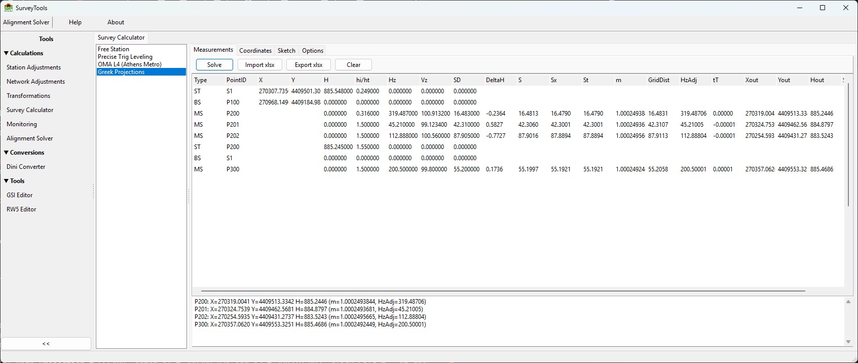
../../_images/Greek_proj1.jpg — The Measurements tab after solving the sample field book: the input columns on the left, the computed columns (DeltaH … Hout, Status) filled in for each solved row, and the per-point results in the panel below.

Note

All angles are in gon (400-gon circle): a zenith of 100 gon is a level sight. Lengths are metres. Decimal point and decimal comma are both accepted in the grids.

2.6.5.2. The field-book model

Work is organised as a field book: an ordered list of rows, each of one of three kinds, entered top to bottom exactly as they were observed.

Type	Meaning
`ST`	Station setup — the point the instrument occupies.
`BS`	Backsight — the reference point the station is oriented to (its horizontal-circle reading).
`MS`	Measurement — a shot to a target point to be computed.

A typical block is one ST row, one BS row, then one or more MS rows. You can then start a new ST block and continue. The calculator solves every block in order.

Chained resolution. Station and backsight rows may either carry explicit coordinates or leave them blank and reference a point by name. Known and computed points share one namespace, so a later station can occupy — or backsight — a point that an earlier measurement computed. This lets you run a short traverse or take side-shots off computed points without re-typing coordinates.

If a station or backsight name cannot be resolved, that block is skipped with an error message; the rest of the field book still solves. A point measured more than once keeps its last solution and raises a warning noting how far the two positions differ.

2.6.5.3. Measurements tab

The Measurements tab holds the field book and the action buttons — Solve, Import, Export xlsx and Clear. Import opens a small menu so you can pick the source format — Excel file… or Geodimeter job file… (more formats will be added over time). Each row has the columns:

Type · PointID · X · Y · H · hi/ht · Hz · Vz · SD

Type edits with an ST / BS / MS drop-down.
X, Y, H — coordinates. On ST/BS rows these are the known coordinates (leave blank to resolve the point by name). On ST rows, H is the station height.
hi/ht — instrument height on an ST row; target height on an MS row.
Hz — the horizontal circle reading (gon). On a BS row it is the reading to the backsight; on an MS row, the reading to the target.
Vz — zenith angle (gon), MS rows only.
SD — slope distance (m), MS rows only.

All calculation settings (projection, radius, refraction, decimals) live on the Options tab described below.

2.6.5.4. What Solve does

For every measurement the engine runs this pipeline (LOCAL applies only the first step; HATT applies the reductions but no scale or t−T):

1. Height difference (with curvature + refraction):
     dH = cos(Vz)·SD
          + ((1-k)/2R)·SD²·sin²(Vz)
          + (SD³·sin²(Vz)·cos(Vz)) / (8R²)
   H  = H_station + hi - ht + dH
2. Horizontal distance:  S = sqrt(SD² - dH²)
3. Reduce to sea level:  Sx = S · R/(R + H_mean)
4. Chord to arc:         St = Sx · (1 + Sx²/24R²)
5. Line-scale factor m   (Simpson-weighted along the line; per projection)
6. Grid distance:        GridDist = St · m
7. Arc-to-chord (t−T) correction of the horizontal angle for both the
   backsight and the target direction  ->  HzAdj
8. Final grid coordinates from the oriented direction and GridDist.

The orientation is derived from the backsight: the grid azimuth station->backsight minus the backsight circle reading gives the reference direction HzRef that every target reading is measured from.

After Solve, the Measurements grid is widened to show the computed columns next to each input row:

DeltaH · S · Sx · St · m · GridDist · HzAdj · tT · Xout · Yout · Hout · Status

The results panel below lists one line per solved point plus any warnings; rows that could not be solved show their reason (unresolved station or backsight, measurement before a setup, zero-length backsight, …).

2.6.5.5. Coordinates tab

The Coordinates tab lists every point in the job — stations and computed points together — as PointID · Kind · X · Y · H, where Kind is Station for occupied points and Point for everything else. Use Export xlsx to write this list to an Excel file.

2.6.5.6. Sketch tab

The Sketch tab is a plan view of the whole job. Stations are drawn as red triangles, points as blue dots, each labelled with its name. Scroll to zoom about the cursor, drag to pan. Export DXF writes the same drawing to a DXF file (stations as triangles, points as circles, names as text) that opens in any CAD package, in real grid coordinates.

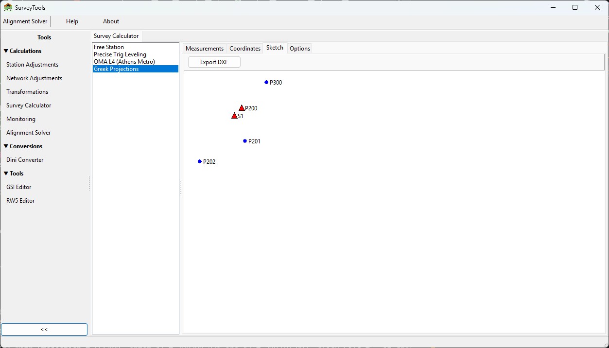
../../_images/Greek_proj2.jpg — The Sketch tab for the sample job: stations `S1` and `P200` as red triangles, computed points `P201`, `P202` and `P300` as blue dots.

2.6.5.7. Options tab

All calculation settings and display options are on the Options tab.

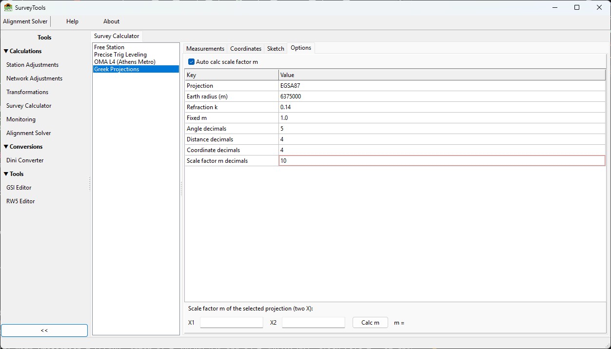
../../_images/Greek_proj3.jpg — The Options tab: the Auto calc m checkbox, the parameter list, the display-decimal settings, and the scale-factor m calculator at the bottom.

Auto calc scale factor m (checkbox, on by default) computes the line-scale factor m automatically for every shot. Clear it to use the fixed value from the Fixed m parameter instead.

Parameters

Key	Default	Meaning
Projection	`EGSA87`	Drop-down: HATT / EGSA87 / TM3 / UTM / LOCAL.
Earth radius (m)	`6375000`	Mean Earth radius used in the reductions.
Refraction k	`0.14`	Coefficient of refraction.
Fixed m	`1.0`	Line-scale factor used when Auto calc m is off.

Display decimals — how many decimal places each kind of value shows in the grids and exports:

Key	Default	Applies to
Angle decimals	`5`	HzAdj and t−T (gon).
Distance decimals	`4`	DeltaH, S, Sx, St, GridDist.
Coordinate decimals	`4`	X, Y, H (Measurements grid and Coordinates tab).
Scale factor m decimals	`10`	the line-scale factor m.

Scale-factor m calculator. At the bottom of the tab, enter two eastings X1 and X2 and press Calc m to get the line-scale factor of the currently selected projection between them (using the Earth radius above and the Scale factor m decimals setting). For example, with EGSA87, X1 = 270307.735 and X2 = 270319.003 gives m = 1.0002493840. HATT and LOCAL always return 1.

2.6.5.8. Import / Export

2.6.5.8.1. Excel workbooks

Import > Excel file… and Export xlsx (Measurements tab) exchange the field book as an .xlsx workbook. The first nine columns are the field book; row 1 is a header and is ignored on import:

Type  PointID   X           Y            H        hi/ht  Hz        Vz        SD
ST    S1        270307.735  4409501.305  885.548  0.249
BS    P100      270968.149  4409184.988                 0.0000
MS    P200                                       0.316  319.4870  100.9132  16.483

Import reads only these nine columns, so a file you exported (which also contains the computed columns) re-imports cleanly.
Point IDs are always kept as text — a purely numeric ID such as 100 survives the round trip unchanged.
Numbers are written as real numeric cells, independent of your Windows regional decimal separator.

A ready-to-use sample workbook is installed at testfiles/EGSA solver/greek_projections_sample.xlsx.

2.6.5.8.2. Geodimeter raw job files

Import > Geodimeter job file… reads a Geodimeter / Trimble .job raw observation file directly into the field book. The file is a plain stream of code=value lines; only the surveying codes are used:

Code	Meaning
`2`	Station (instrument) point number — starts an `ST` row.
`3`	Instrument height of that station (`hi`).
`62`	Backsight / reference point number — starts a `BS` row.
`5`	Target point number — starts an `MS` row.
`7` / `8` / `9`	Horizontal circle (`Hz`), zenith angle (`Vz`) and slope distance (`SD`), in gon and metres.
`6`	Reflector (target) height.
`21` / `4` / `50`	Reference angle, feature code and job name — read but not used.

Two conventions are worth knowing:

Reflector height (code 6) is a running setting: each shot uses the last 6 value seen in its own record, and a shot with no 6 of its own keeps the previous height.
The backsight direction is taken from the measured reading (code 7), not from the reference angle (code 21).

Important

A .job file contains no coordinates — only station names and raw readings. After importing, type the known X, Y, H of the first station and its backsight into their ST / BS rows, then Solve. Every later setup occupies a point measured from an earlier one, so its coordinates and its height are resolved automatically by chaining; you only supply the initial control. All coordinates you type — including a backsight’s height — appear in the Coordinates tab alongside the computed points.

A sample job is installed at demo_files\SurveyCalculator\GreekProjections\test_geodimeter.job.

2.6.5.9. Worked example

Set Projection = EGSA87 and Solve the sample workbook (or type the rows below). It is a two-setup job: a station S1 with three side shots, then a second setup that occupies the computed point P200 and backsights the known S1.

Type  PointID  X           Y            H        hi/ht  Hz        Vz        SD
ST    S1       270307.735  4409501.305  885.548  0.249
BS    P100     270968.149  4409184.988                 0.0000
MS    P200                                       0.316  319.4870  100.9132  16.483
MS    P201                                       1.500  45.2100   99.1234   42.310
MS    P202                                       1.500  112.8880  100.5600  87.905
ST    P200                              885.245  1.550                              (occupies computed P200)
BS    S1                                                0.0000                       (backsight known S1)
MS    P300                                       1.500  200.5000  99.8000   55.200

Expected results (EGSA87, R = 6 375 000, k = 0.14):

Point	X	Y	H
P200	270319.004	4409513.334	885.245
P201	270324.754	4409462.568	884.880
P202	270254.593	4409431.274	883.524
P300	270357.062	4409553.325	885.469

Open the Coordinates tab to see all five points (S1 and P200 marked Station), and the Sketch tab for the plan view.

2.6.5.10. Projection constants and notes

Projection	m0	False easting
HATT	1.0	0
EGSA87	0.9996	500 000
TM3	0.9999	200 000
UTM	0.9996	500 000
LOCAL	1.0	0

Coordinate convention. X is the easting-type coordinate, Y the northing; both are the grid values as stored in your project.
Parity with Provolika. The engine reproduces the original tool exactly, including its arc-to-chord formulation and the fixed UTM constants (the same m0 and false easting are used regardless of zone). No atmospheric (pressure/temperature) correction is applied — as in the original.
HATT and LOCAL. HATT applies the height, sea-level and arc reductions but no scale factor (m = 1) and no t−T correction. LOCAL treats the data as a plane job: height difference only, no projection reductions.
Reusable engine. The calculations live in the IQcalc engine (iqcalc.provolika and iqcalc.provolika.fieldbook) and can be reused by other software independently of this tool.