2.1.1. Station Adjustment

2.1.1.1. Overview

The Station Adjustment module performs least-squares adjustment of survey observations collected at instrument stations. It processes horizontal angles, vertical (zenith) angles, and slope distances measured in multiple face and cycle sets, producing adjusted directions, adjusted angles, adjusted distances, and comprehensive statistical quality indicators.

The module supports multi-station projects — all stations from a survey campaign are stored in a single .adjproj project file (SQLite database), allowing batch processing, cross-station analysis, and network overview reporting.

All angles are in gradians (400 grads per full circle). Angle residuals are expressed in centesimal seconds (cc) where 1 grad = 10000 cc. Distance residuals are in millimeters (mm).

2.1.1.2. Getting Started

2.1.1.2.1. Opening the Module

Open the Station Adjustment module from the sidebar under Calculations > Station Adjustments. The module opens as a separate window.

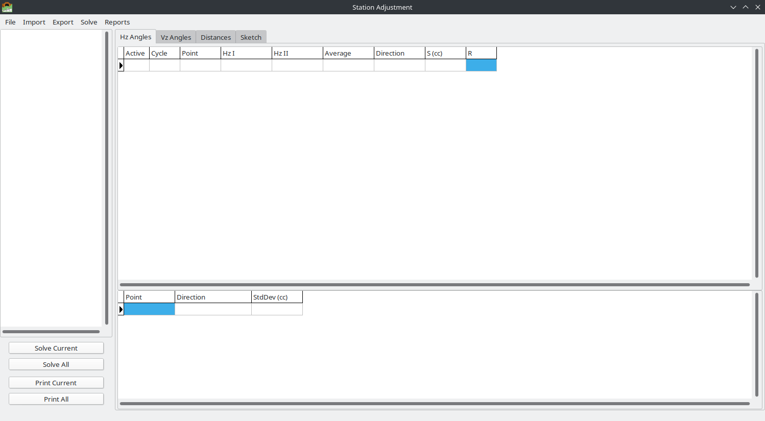
Station Adjustment main window (empty state)

The Station Adjustment window in its initial empty state.

2.1.1.2.2. Creating a New Project

Go to File > New Project
Choose a location and filename (extension .adjproj)
If the file already exists, you will be asked to confirm overwrite
The project is created as an empty SQLite database ready to receive observations

2.1.1.2.3. Opening an Existing Project

Go to File > Open Project
Select an existing .adjproj file
The station tree on the left will populate with all stored stations

Note

Each time the Station Adjustment window is opened, it starts with an empty state. You must create or open a project before importing data.

2.1.1.3. Importing Observations

The module supports multiple import formats for survey observations.

2.1.1.3.1. Import from Leica LandXML

File > Import > LandXML…

Imports raw observations from Leica Captivate LandXML export files (.xml). This is the recommended import method for Leica total station data.

Supported data from LandXML:

Station setups with instrument height (<InstrumentSetup>)
Raw horizontal angles, zenith angles, and slope distances (<RawObservation>)
Face I and Face II observations (directFace attribute)
Target point names and target heights (<TargetPoint>)
Automatic cycle detection from Face I/II grouping
Multiple stations per file

How Leica LandXML data is structured:

The Leica Captivate software exports survey jobs in LandXML 1.2 format. The key elements are:

LandXML structure (simplified)

<LandXML version="1.2">
  <Units>
    <Metric angularUnit="grads" linearUnit="meter"/>
  </Units>
  <Survey>
    <InstrumentSetup id="TPSSetupID_3_11"
                     stationName="30001"
                     instrumentHeight="0.237">
      <InstrumentPoint>...</InstrumentPoint>
    </InstrumentSetup>
    ...
    <ObservationGroup id="oTPSSetupID_3_11">
      <RawObservation setupID="TPSSetupID_3_11"
                      horizAngle="315.506830..."
                      zenithAngle="97.012060..."
                      slopeDistance="54.002900"
                      targetHeight="0.237"
                      directFace="true">
        <TargetPoint name="30002"/>
      </RawObservation>
      ...
    </ObservationGroup>
  </Survey>
</LandXML>

Key attributes:

Attribute	Description
`stationName`	Name of the instrument station (from `<InstrumentSetup>`)
`instrumentHeight`	Height of instrument above the station mark (meters)
`horizAngle`	Horizontal angle reading (gradians)
`zenithAngle`	Zenith angle reading (gradians, 100 = horizontal)
`slopeDistance`	Slope distance (meters)
`targetHeight`	Height of target/prism above the target point (meters)
`directFace`	`true` = Face I (direct), `false` = Face II (reverse)
`purpose`	`backsight` = orientation shot (skipped), `normal` = measurement

Face I / Face II pairing:

The importer automatically pairs Face I and Face II observations for the same target point within the same measurement cycle. Leica instruments typically record observations in this pattern:

Face I:  Point A, Point B, Point C, Point D
Face II: Point D, Point C, Point B, Point A  (reverse order)
Face I:  Point A, Point B, Point C, Point D  (next cycle)
...

Each pair produces one observation record with both Face Left (Face I) and Face Right (Face II) values.

Backsight observations (purpose="backsight") are automatically skipped — they represent the station orientation shot, not a measurement set observation.

Note

For detailed information about the Leica LandXML format, refer to:

Leica Captivate Technical Reference Manual — Leica Geosystems AG
LandXML 1.2 Schema Specification — http://www.landxml.org/schema/LandXML-1.2/
Leica Captivate LandXML Export documentation from your instrument software

2.1.1.3.2. Import from Leica GSI

File > Import > Leica GSI…

Imports observations from Leica GSI8 or GSI16 format files (.gsi). The GSI parser automatically detects the format version and extracts horizontal angles, vertical angles, slope distances, point names, and target heights.

About the Leica GSI Format:

GSI (GEO Serial Interface) is an ASCII text format used by Leica total stations (TPS series) and digital levels (DNA series). Each line contains one measurement record composed of space-separated data words. Two variants exist:

GSI8 — 8-character data fields (older instruments)
GSI16 — 16-character data fields (modern instruments, supports large coordinates and long point names)

Data word structure:

Each word in a GSI line follows this positional format:

WW.XYZS DDDDDDDDDDDDDDDD
||  |||  |
||  |||  +-- Data (8 chars for GSI8, 16 chars for GSI16)
||  ||+----- Sign (+ or -)
||  |+------ Units/decimal indicator
||  +------- Input mode (0=measured, 1=keyboard, 2=corrected)
|+---------- Auto-index info
+----------- Word Index (WI) — identifies the data type

Word Index (WI) codes used by the importer:

WI	Name	Description
11	Point Number	Target point name (alphanumeric, right-padded with zeros)
21	Horizontal Angle (Hz)	Horizontal circle reading (gradians)
22	Vertical Angle (V)	Zenith angle reading (gradians, 100 = horizontal)
31	Slope Distance	Slope distance (meters)
32	Horizontal Distance	Horizontal distance (meters)
33	Height Difference	Height difference between instrument and target (meters)
51	PPM / Constants	Parts per million and prism constant
81	Target Easting	Easting coordinate of target point (meters)
82	Target Northing	Northing coordinate of target point (meters)
83	Target Elevation	Elevation of target point (meters)
84	Station Easting	Easting coordinate of instrument station (meters)
85	Station Northing	Northing coordinate of instrument station (meters)
86	Station Elevation	Elevation of instrument station (meters)
87	Reflector Height	Height of target/prism above ground mark (meters)
88	Instrument Height	Height of instrument above station mark (meters)

Units indicator (position 6 in each word):

Code	Unit	Decimal places
0	Meters (mm precision)	3
2	Gradians (gon)	5
6	Meters (1/10 mm precision)	4
8	Meters (1/100 mm precision)	5

GSI16 sample — observation line:

GSI16 file sample with field breakdown

*110005+00000000000000T5 21.322+0000000034921514 22.322+0000000007636738 31..06+0000000000791854 87..16+0000000000002530
 |   |  |              |  | ||   |                |  |                     |                      |
 |   |  |              |  | ||   |                |  |Vz=76.36738 gon      |Sd=79.1854 m          |Ht=0.2530 m
 |   |  |              |  | ||   |                |Hz=349.21514 gon
 |   |  |              |  | ||   +-- 5 decimals (gon)
 |   |  |              |  | |+-- measured
 |   |  |              |  | +--- compensator active
 |   |  |              |  +-- WI 21 (Horizontal Angle)
 |   |  |Point name: T5
 |   +- Line number: 0005
 +-- WI 11 (Point Number), * marks first word

Station setup record (when present):

Some Leica instruments record a station setup line before observations begin, containing WI 84/85/86 (station coordinates) and WI 88 (instrument height):

Station setup record in GSI16

*110001+000000000MBM1PB1 84..16+0000000000000000 85..16+0000000000000000 86..16+0000000000000000 88..16+0000000000016010
 |                       |Station E=0.0000        |Station N=0.0000        |Station H=0.0000        |Hi=1.6010 m

A station setup line is identified by the presence of WI 84 and the absence of angle fields (WI 21, 22). The point name in WI 11 gives the station name.

Note

Not all instruments or configurations output station setup records. When station setup records are absent, the importer creates a station name from the filename. The importer also skips Leica “Set of Angles” result lines (WI 41, identified by names like HZ-RESLT, HZ-MEAN0, HZ-DIFF0) which contain the instrument’s internal averaging results.

Face I / Face II detection:

The GSI format does not have an explicit face indicator. Face I vs Face II is determined from the vertical angle:

Vz < 200 gon — Face I (direct)
Vz >= 200 gon — Face II (reverse)

Observations are paired into cycles based on the point sequence pattern (Face I forward, Face II reverse).

Note

For detailed information about the Leica GSI format, refer to:

Leica Geosystems — GSI Online for Leica TPS — Official GSI format documentation
Total Open Station — https://totalopenstation.readthedocs.io/en/stable/input_formats/if_leica_gsi.html — Open-source GSI format reference

2.1.1.3.3. Import from Legacy SAJ Project

File > Import > Legacy Project (.saj)…

Imports station adjustment data from the legacy .saj format (used by earlier versions of SurveyTools). This XML format stores pre-organized observations with Face I, Face II, and cycle information.

2.1.1.3.4. Import from Spreadsheet (Excel/CSV)

File > Import > Spreadsheet (Excel/CSV)…

Opens the Import Wizard — a 3-step process for importing observations from Excel (.xlsx, .xls) or CSV files.

Step 1 — File Selection:

Select the spreadsheet file
For multi-sheet Excel files, choose the sheet to import
Check/uncheck “First row contains headers” (auto-detected)
Preview the first 20 rows of data

Step 2 — Column Mapping:

Map spreadsheet columns to observation fields using dropdown selectors:

Field	Required	Description
Station Name	Yes	Name of the instrument station
Point Name	Yes	Name of the target point
Cycle / Set	No	Measurement cycle number (defaults to 1 if not mapped)
Hz Face I	Yes	Horizontal angle, Face I reading (gradians)
Hz Face II	No	Horizontal angle, Face II reading (gradians)
Vz Face I	No	Zenith angle, Face I reading (gradians)
Vz Face II	No	Zenith angle, Face II reading (gradians)
Dist Face I	No	Slope distance, Face I reading (meters)
Dist Face II	No	Slope distance, Face II reading (meters)
Target Height	No	Height of target/prism (meters)
Instrument Height	No	Height of instrument (meters)

The wizard auto-detects column mappings when headers match common patterns (e.g., “Station”, “Hz1”, “Vz_I”, “SlopeDist”).

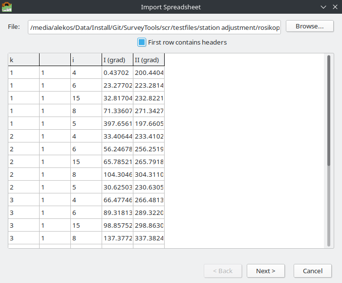
Import Wizard — Step 1: File selection and preview

Import Wizard Step 1 — File selection with data preview.

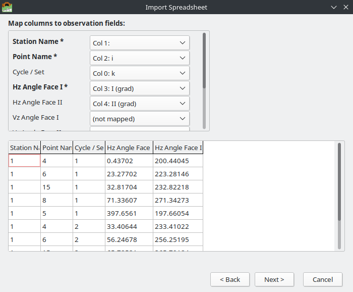
Import Wizard Step 2 — Column mapping with mapped data preview.

Step 3 — Summary & Import:

Review the number of stations and observations detected, then click Import to add the data to the project.

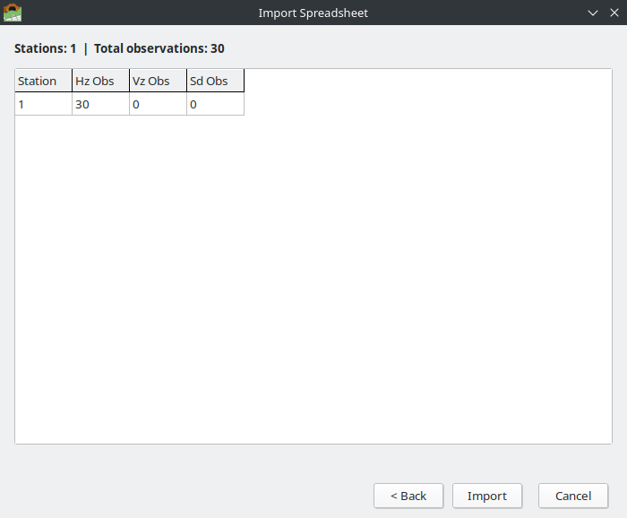
Import Wizard — Step 3: Summary and import

Import Wizard Step 3 — Summary showing station and observation counts.

2.1.1.3.5. Import ASCII Files

File > Import > ASCII Horizontal Angles / Vertical Angles / Slope Distances

Import observations from simple comma-separated text files. Each observation type has its own file format:

Horizontal angles: Set,Point,Hz1,Hz2

Horizontal angles file sample

1,T5,349.21514,149.21431
1,T6,41.08037,241.08152
1,T2,173.64603,373.64667
2,T5,349.21646,149.21488

Vertical angles: Set,Point,Vz1,Vz2

Vertical angles file sample

1,T5,76.36738,323.63154
1,T6,72.62374,327.37370

Slope distances: Set,Point,Sd1,Sd2,TargetHeight

Slope distances file sample

1,T5,79.1854,79.1855,0
1,T6,56.8387,56.8385,0

2.1.1.4. Working with Observations

2.1.1.4.1. Station Tree

The left panel shows all stations in the project as a tree view. After solving, each station shows its quality indicator:

Station Name (S=2.72cc) — solved station with standard deviation of unit weight
Station Name (S=165.93cc) [!] — station with outlier observations flagged

Click a station to view its observations and results.

Right-click a station for the context menu: Rename, Delete, Solve, Print Combined.

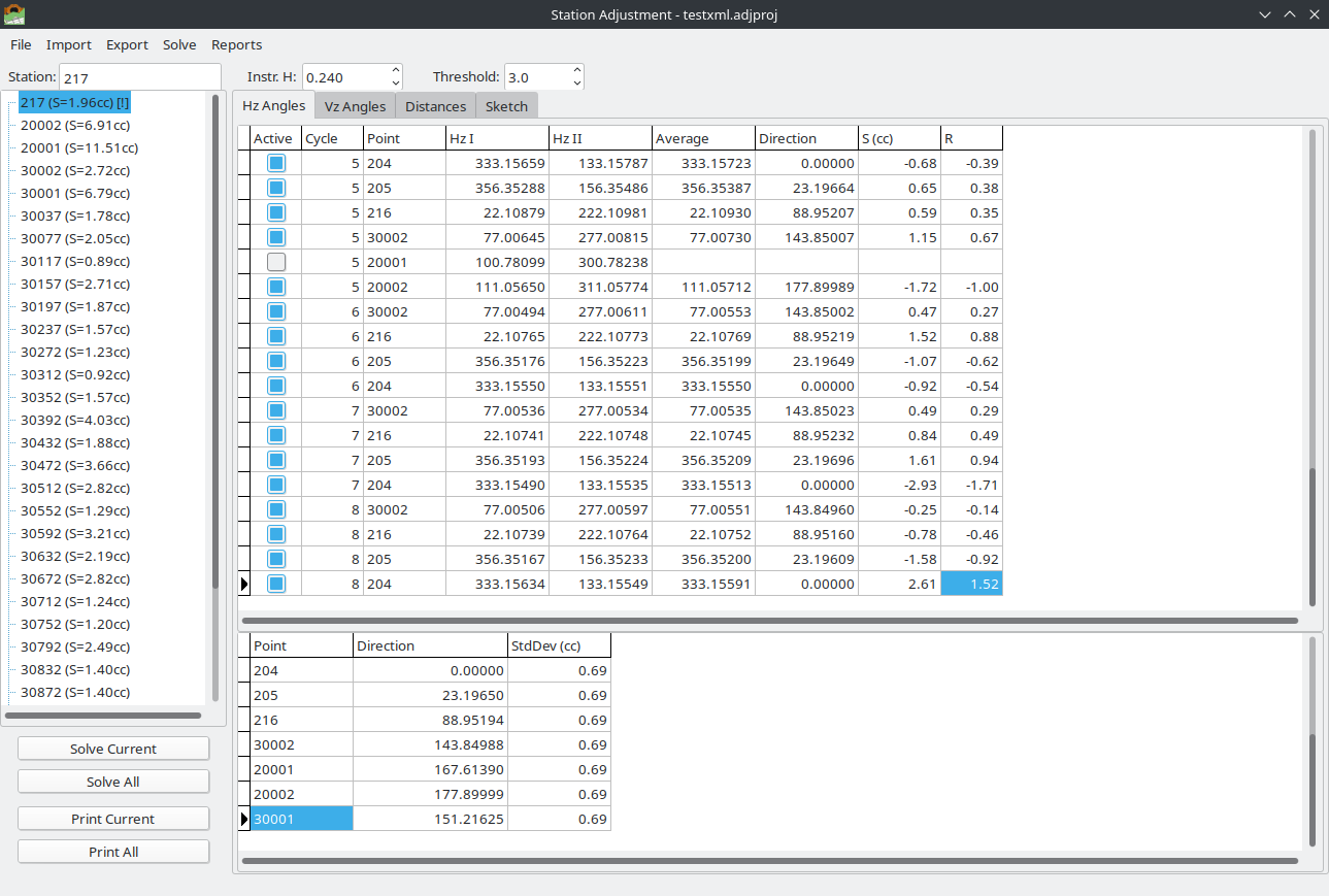
Station tree showing solved stations with S-value quality indicators.

2.1.1.4.2. Observation Tabs

The main area has four tabs:

Hz Angles — horizontal angle observations and adjusted directions
Vz Angles — vertical/zenith angle observations and adjusted angles
Distances — slope distance observations and adjusted distances
Sketch — geometric visualization (Station View or Network View)

Each observation tab shows two grids:

Raw Measurements (top) — all raw observations with Face I, Face II, averages, and computed residuals (S, R, T)
Adjusted Results (bottom) — adjusted values with standard deviations per point

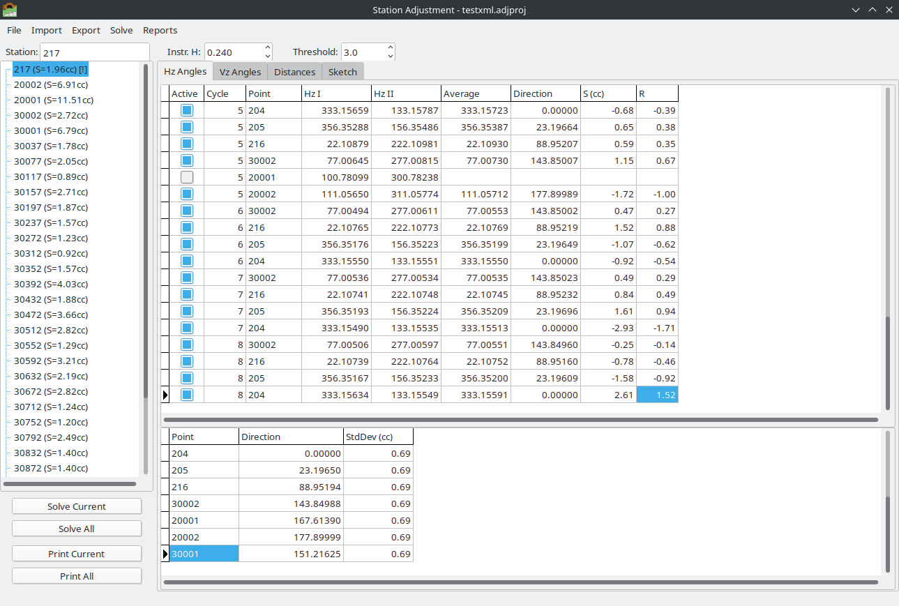
Horizontal angles tab with adjusted results and measurements

Horizontal Angles tab showing raw measurements with residuals (top grid) and adjusted directions (bottom grid).

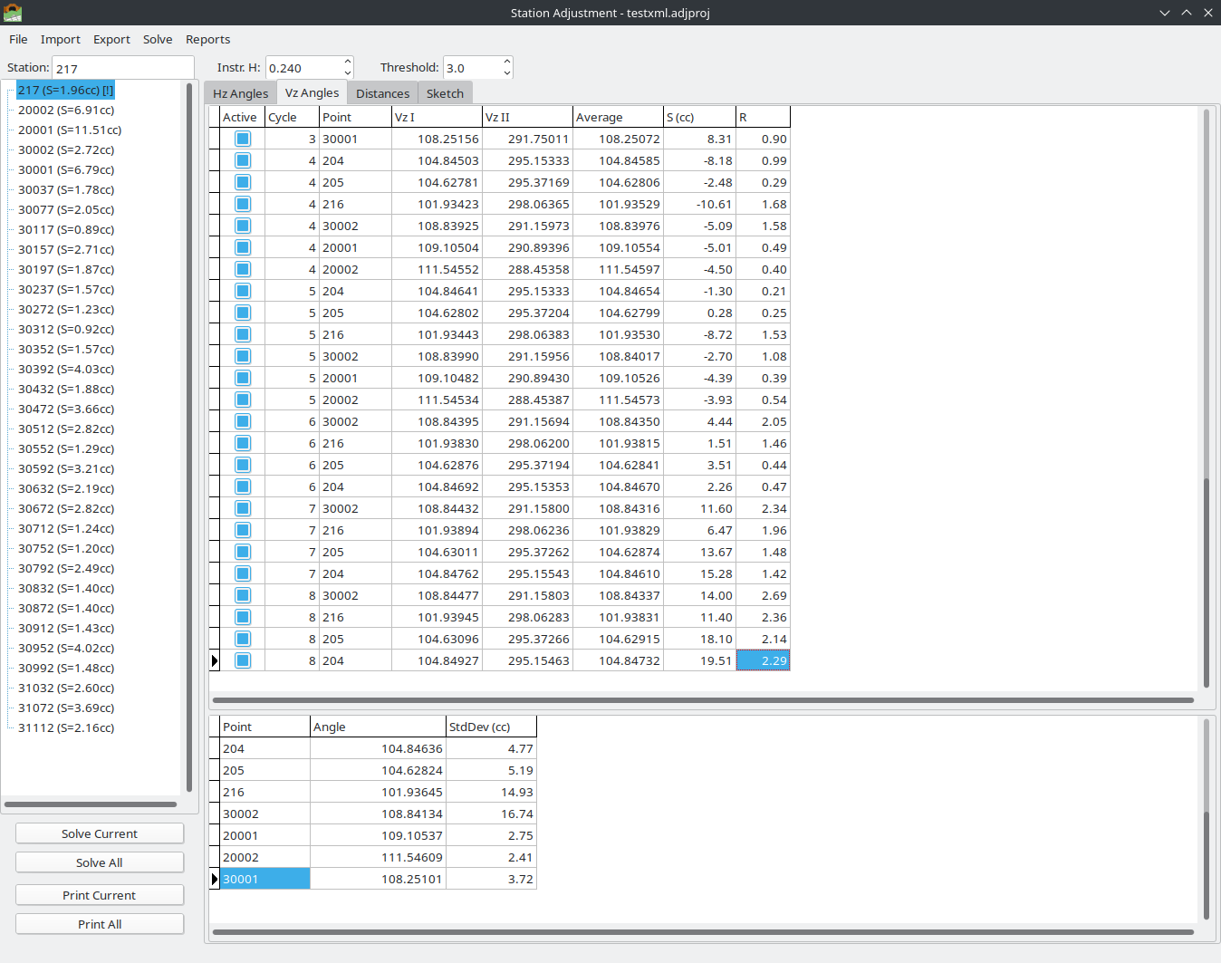
Vertical Angles tab showing raw measurements (top) and adjusted zenith angles (bottom).

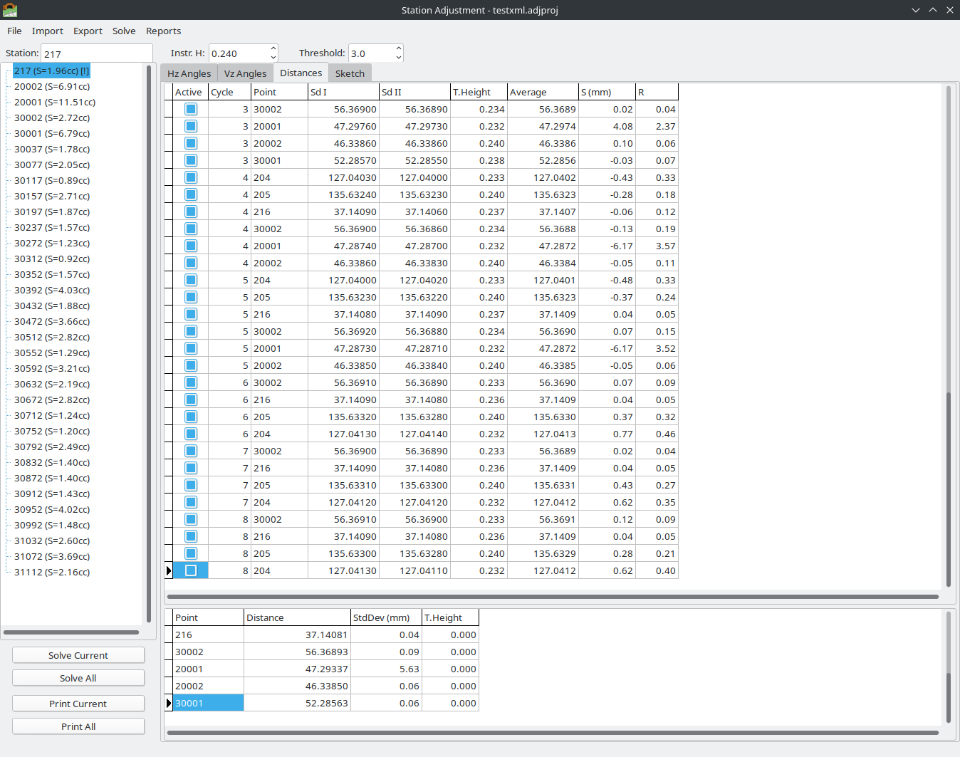
Slope Distances tab showing raw measurements (top) and adjusted distances with standard deviations (bottom).

Editing observations:

Click the Active column checkbox to activate/deactivate individual observations
Deactivated observations are excluded from the adjustment
Face I and Face II values can be edited directly in the grid

2.1.1.4.3. Reorder Points

Solve > Reorder Points…

Opens a dialog to change the order of observed points. This affects the order in all cycles simultaneously and is applied to Hz, Vz, and Sd observations.

Use Up / Down buttons to manually reorder
Use Sort A-Z / Sort Z-A for automatic alphabetical sorting

This is useful when imported data has points in an inconvenient order.

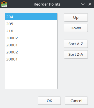
Reorder Points dialog with manual Up/Down and automatic sorting options.

2.1.1.4.4. Station Information

The station info panel (below the tree) shows:

Station Name — editable
Instrument Height — editable (meters)
Outlier Threshold — the T-value threshold for outlier detection (default: 3.0)

2.1.1.5. Solving (Adjustment)

2.1.1.5.1. Solve Current Station

Solve > Solve Current Station

Performs least-squares adjustment for the selected station. The adjustment processes horizontal angles, vertical angles, and slope distances independently.

2.1.1.5.2. Solve All Stations

Solve > Solve All Stations

Performs adjustment for every station in the project.

2.1.1.5.3. Deactivate Outliers

Solve > Deactivate Outliers & Re-solve

Opens the Outlier Review Dialog — an interactive two-phase tool for reviewing and selectively deactivating observations flagged as outliers (|R| > threshold).

Phase 1 — Review Checklist:

The dialog shows all flagged outlier observations in a checklist, sorted by R-value (worst first). For each outlier, the following information is displayed:

Type — observation type (HZ, VZ, SD)
Point — target point name
Cycle — measurement cycle number
Face Left / Face Right — original face readings
Average — face-averaged value
Residual — deviation from adjusted value (cc for angles, mm for distances)
R-value — standardized residual (dimensionless)

All outliers are pre-checked for deactivation. Uncheck any observations you want to keep active. Click Deactivate Selected to proceed, or Cancel to abort.

Phase 2 — Before/After Comparison:

After deactivation and re-solving, the dialog shows a statistics comparison for each affected observation type:

Statistic	Before	After	Change
S² (variance factor)	2.410	1.080	-55.2%
Sv (std. deviation)	1.553	1.040	-33.0%
Max Residual	4.210	1.890	-55.1%
Obs Count	48	45	-3

The comparison helps assess whether the deactivation improved the adjustment quality.

Available actions in Phase 2:

Undo — re-activates the deactivated observations and re-solves, returning to Phase 1
Review New Outliers — if new outliers appeared after re-solving (because the adjustment shifted), opens Phase 1 again for the new outliers. This chaining continues up to 5 iterations.
Close — accepts the result and closes the dialog

After closing, the station tree automatically updates to reflect the new S-value and outlier status.

2.1.1.5.4. Complete vs. Incomplete Observation Sets

The adjustment engine automatically detects whether the observation set is complete or incomplete and selects the appropriate solver.

Complete sets — every target point has observations in every cycle, and both Face I and Face II are present for all observations. This is the ideal case and uses the classical direction adjustment method with full matrix formulation.

Incomplete sets — one or more of the following conditions exist:

A target point is missing in one or more cycles (e.g., point was not visible during that cycle)
An observation has only Face I or only Face II (single-face observation)
Different points have different numbers of cycles

The engine handles incomplete sets using a generalized least-squares approach:

Single-face observations: When only Face I is available, the face reading is used directly as the average. When only Face II is available, the reading is corrected by 200 grads (half-turn) to convert it to the equivalent Face I reading. Both cases are included in the adjustment.
Missing cycles: Points with fewer cycles than others are still adjusted — the solver uses all available observations regardless of completeness.
Mixed data: The solver builds the design matrix from whatever observations are available, computing the normal equations and solving for the direction unknowns.

Note

When incomplete sets are detected, the solver automatically switches to the SolveIncomplete method. This is transparent to the user — the same Solve command handles both cases. The degrees of freedom and statistics are computed correctly for the actual number of observations present.

2.1.1.6. Calculation Method — Detailed Explanation

This section explains the mathematical procedures used in the station adjustment. Understanding these methods helps surveyors interpret the results and assess observation quality.

2.1.1.6.1. Horizontal Angle Adjustment

Objective: Determine the most probable adjusted directions to each target point from the station, using all available face and cycle observations.

Step 1 — Face Averaging

For each observation with both Face I and Face II readings, the face average is computed:

\[\bar{Hz} = \frac{Hz_I + Hz_{II} \pm 200}{2}\]

The sign depends on whether Hz_I is greater or less than 200 grads. This eliminates the systematic collimation error (2c) of the instrument. If only one face is available, that reading is used directly (or corrected by 200g for Face II only).

Step 2 — Reduced Directions

For each cycle, a reference point (typically the first point observed) is chosen. All face-averaged readings in that cycle are reduced by subtracting the reference reading:

\[d_i = \bar{Hz}_i - \bar{Hz}_{ref}\]

This removes the orientation unknown for each cycle, producing reduced directions that are comparable across cycles.

Step 3 — Design Matrix and Normal Equations

The adjustment uses the method of observation equations. The unknowns are:

(p - 1) direction unknowns — one for each target point except the reference point (fixed to 0)
c orientation unknowns — one for each measurement cycle

The observation equation for the i-th observation is:

\[v_i = d_i - x_{point} + z_{cycle}\]

where: - v_i is the residual - x_point is the direction unknown for the target point - z_cycle is the orientation unknown for the cycle

This is assembled into matrix form: v = A·x - b, where A is the design matrix, x is the vector of unknowns, and b is the vector of reduced directions.

Step 4 — Least Squares Solution

The normal equations are formed and solved:

\[N = A^T \cdot A\]

\[u = A^T \cdot b\]

\[x = N^{-1} \cdot u\]

The matrix N is inverted using ALGLIB’s matrix inversion routines.

Step 5 — Residuals and Statistics

Residuals are computed as:

\[v = b - A \cdot x\]

The a-posteriori variance of unit weight (S² a posteriori) is:

\[S^2_0 = \frac{v^T \cdot v}{f}\]

where f is the degrees of freedom:

\[f = n - p - c + 1\]

with n = number of observations, p = number of points, c = number of cycles.

The standard deviation of unit weight is:

\[S_0 = \sqrt{S^2_0}\]

reported in centesimal seconds (cc), where 1 grad = 10,000 cc.

The standard deviation of adjusted directions (Sv) is:

\[S_v = \sqrt{S^2_0 \cdot \frac{n - p - c + 5}{n}}\]

Step 6 — Standard Deviation of Adjusted Values

The standard deviation of each adjusted direction (Sdev) is derived from the diagonal elements of the cofactor matrix and the a-posteriori variance:

\[\sigma_{x_i} = S_0 \cdot \sqrt{Q_{ii}}\]

where Q_ii is the diagonal element of \(N^{-1}\) corresponding to direction i.

All Sdev values are reported in centesimal seconds (cc) in both the grid display and the printed report.

2.1.1.6.2. Vertical Angle (Zenith) Adjustment

Objective: Determine the most probable zenith angle to each target point, with correction for the instrument’s collimation index error.

Step 1 — Face Averaging

For dual-face observations, the zenith average is:

\[\bar{Vz} = \frac{Vz_I - Vz_{II} + 400}{2}\]

This formula removes the collimation index error. For single-face observations, the reading is used directly (Face II is converted via 400 - Vz_II).

Step 2 — Collimation Index

The collimation index (systematic vertical circle error) is computed from all dual-face observations:

\[c_i = \frac{Vz_{I,i} + Vz_{II,i} - 400}{2}\]

\[z = \frac{\sum c_i}{n_{dual}}\]

where n_dual is the number of observations with both faces.

Step 3 — Adjusted Zenith Angles

For each target point, the adjusted zenith angle is the mean of all face-averaged values across cycles:

\[\bar{Vz}_{point} = \frac{\sum_{cycles} \bar{Vz}_i}{n_{cycles}}\]

Step 4 — Residuals

For dual-face observations, two residuals are computed per observation:

\[v_{1,i} = Vz_{I,i} - \bar{Vz}_{point} - z\]

\[v_{2,i} = (400 - Vz_{II,i}) - \bar{Vz}_{point} + z\]

For single-face observations, only one residual is computed.

Step 5 — Statistics

The degrees of freedom account for both face residuals:

\[f = n_{equations} - p\]

where n_equations counts each face as a separate equation (dual-face observations contribute 2 equations, single-face contributes 1).

The a-posteriori variance and standard deviation are computed as for horizontal angles, with residuals in cc.

2.1.1.6.3. Slope Distance Adjustment

Objective: Determine the most probable slope distance to each target point, with correction for systematic instrument bias.

Step 1 — Face Averaging

For dual-face distance observations:

\[\bar{Sd} = \frac{Sd_I + Sd_{II}}{2}\]

For single-face observations, the available reading is used directly.

Step 2 — Systematic Bias

A systematic bias (instrument constant error) is estimated:

\[z = \frac{\sum (Sd_{I,i} - Sd_{II,i})}{2 \cdot n_{dual}}\]

This represents the systematic difference between Face I and Face II distance readings.

Step 3 — Adjusted Distances

For each target point, the adjusted distance is the mean of all face-averaged values:

\[\bar{Sd}_{point} = \frac{\sum_{cycles} \bar{Sd}_i}{n_{cycles}}\]

Step 4 — Residuals

Similar to zenith angles, face residuals are computed:

\[v_{1,i} = Sd_{I,i} - \bar{Sd}_{point} - z\]

\[v_{2,i} = Sd_{II,i} - \bar{Sd}_{point} + z\]

Step 5 — Statistics

The a-posteriori variance and standard deviation are computed in mm² and mm respectively. Degrees of freedom follow the same logic as for vertical angles.

2.1.1.6.4. Outlier Detection

Standardized Residual (R):

The R-value normalizes each residual by the standard deviation of unit weight:

\[R_i = \frac{v_i}{S_0}\]

Observations with |R| > threshold (default 3.0) are flagged as potential outliers.

T-test Value:

The T-value provides a more robust outlier test using the Student’s t-distribution:

\[T_i = R_i \cdot \sqrt{\frac{f - 1}{f - R_i^2}}\]

where f is the degrees of freedom. Large T-values indicate observations that are statistically inconsistent with the rest of the data set.

Interactive Outlier Review:

Use Solve > Deactivate Outliers & Re-solve to open the Outlier Review Dialog (see Deactivate Outliers above). The dialog shows each flagged observation with its details, allowing you to selectively deactivate specific outliers while keeping others. After deactivation, a before/after statistics comparison shows how the adjustment improved.

Warning

Always review outliers before deactivating them. An outlier may indicate a real problem (wrong target, instrument error) or it may be a valid observation in a noisy dataset. Blindly removing outliers can bias the adjustment.

2.1.1.6.5. Understanding the Results

Measurements table (top grid) — Horizontal Angles:

Column	Description
Set	Measurement cycle number
Point	Target point name
Hor. Angle (I)	Face I horizontal reading (gradians)
Hor. Angle (II)	Face II horizontal reading (gradians)
Average	Face-averaged horizontal reading
Direction	Reduced direction (relative to reference point)
S (cc)	Residual in centesimal seconds
R	Standardized residual (dimensionless)
T	T-test value for outlier detection

Adjusted Results table (bottom grid):

Column	Description
Point	Target point name
Direction / Angle / Distance	Adjusted value (gradians for angles, meters for distances)
Sdev (cc / mm)	Standard deviation of the adjusted value

Statistical Summary (footer area):

Statistic	Description
S² a posteriori	A-posteriori variance of unit weight (cc² for angles, mm² for distances). Ideally close to 1.0 when using calibrated instruments with correct a-priori weights.
Std.Dev. unit weight (S)	Standard deviation of unit weight (cc or mm). This is the primary quality indicator — lower values indicate better precision.
Std.Dev. directions (Sv)	Standard deviation of adjusted directions (cc, Hz only). Represents the expected precision of each adjusted direction.
Degrees of freedom	Number of redundant observations (f = observations - unknowns). Must be >= 1 for the adjustment to produce meaningful statistics. Higher values provide more reliable statistical tests.

Interpreting S₀ (Standard Deviation of Unit Weight):

S₀ < 5 cc — Excellent precision, typical for high-end total stations with careful observation procedures
S₀ = 5-15 cc — Good precision, normal for routine survey work
S₀ = 15-50 cc — Moderate precision, may indicate difficult conditions or lower instrument accuracy
S₀ > 50 cc — Poor precision, investigate potential problems (unstable setup, atmospheric disturbance, wrong targets)

2.1.1.7. Reports

Reports > Current Station — Hz Angles / Vz Angles / Distances / Combined

Generates printable reports for the selected station with:

Adjusted results table
Full measurement table with residuals
Statistical summary (S², S, Sv, degrees of freedom)
Station sketch (geometric visualization of observed points)

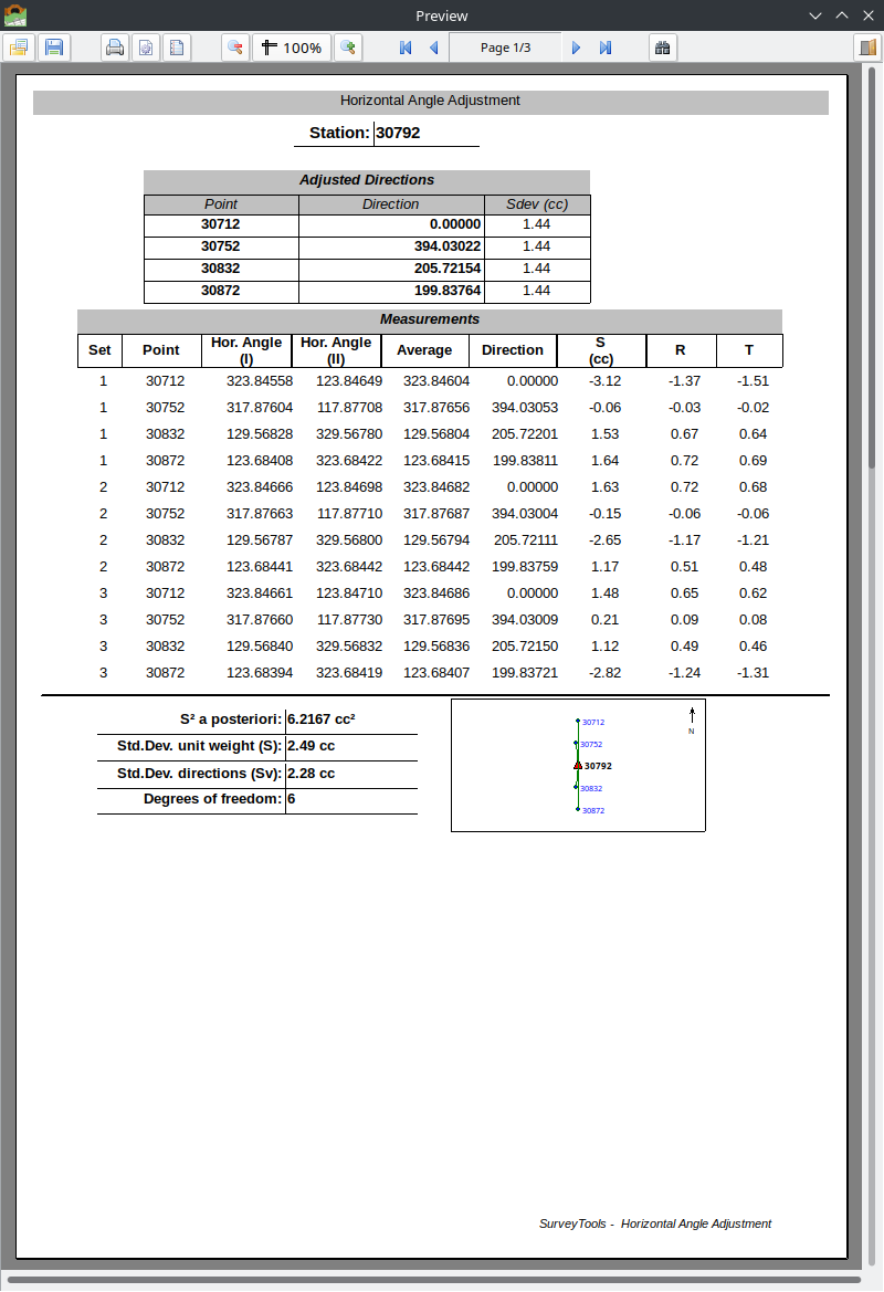
Horizontal Angle Adjustment report with adjusted directions, measurements, statistics, and station sketch.

Reports > All Stations — Combined

Generates a batch report for all stations, with a Network Overview page showing the full survey network geometry.

The network overview is a portrait-orientation page showing all stations (colored triangles) and observed points (blue dots) with observation lines.

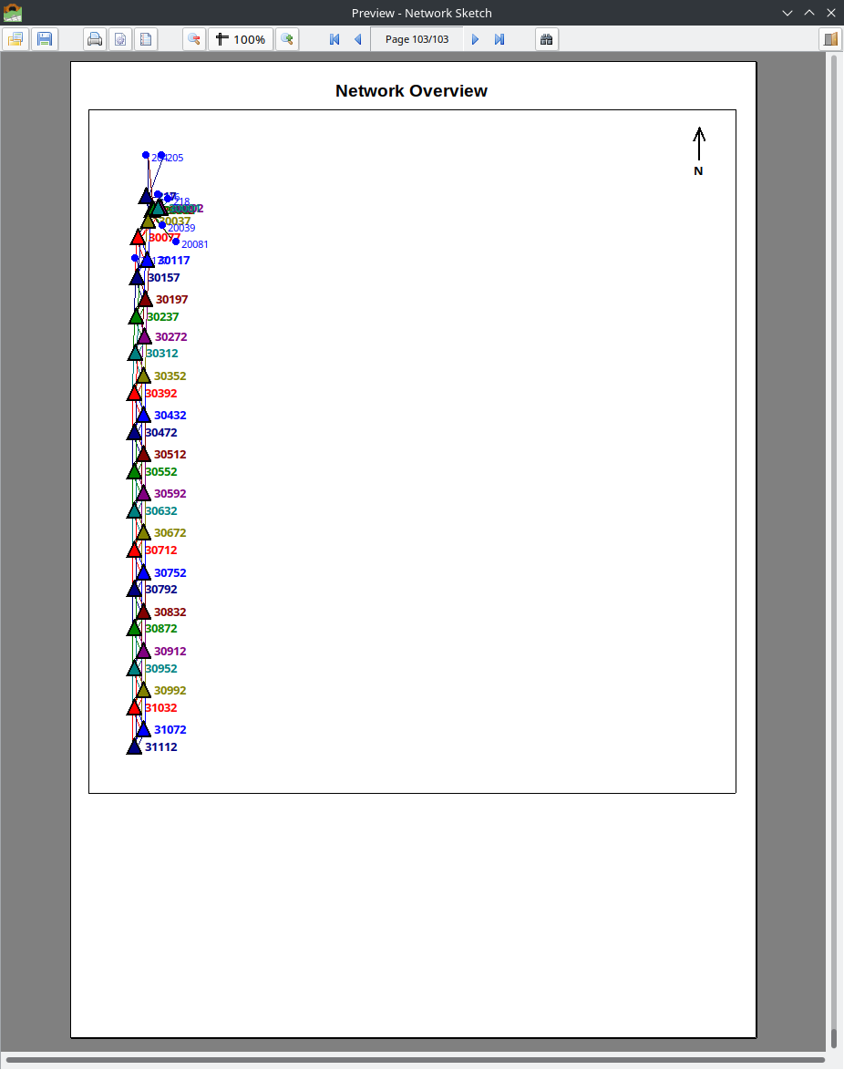
Network Overview page showing the complete survey network geometry.

2.1.1.8. Exporting Data

2.1.1.8.1. Export Adjusted Measurements

Export > Adjusted Measurements > All / Hz Angles / Vz Angles / Distances

Exports adjusted values for all stations to CSV format.

All adjusted measurements export format

Station,Instrument Height,Point,H Angle,H Angle Sdev,Point,V.Angle,V angle sdev,Point,Slope dist,Slope Dist Sdev,Target height
30001,0.237,217,0.00000,1.57,217,91.75228,2.82,217,56.3683,0.00,0.239
30001,0.237,30002,339.83624,1.57,218,91.86066,3.51,30001,7.4624,0.03,0.239

2.1.1.8.2. Export Raw Data

Export > Raw Data > All / Hz Angles / Vz Angles / Distances

Exports the original (unadjusted) observation data for all stations to CSV format.

2.1.1.8.3. Export to Starnet

Export > 3rd Party > Starnet…

Exports adjusted observations in STAR*NET format (.dat) for use in MicroSurvey STAR*NET or compatible network adjustment software.

The exported file uses:

.UNITS GONS — angles in gradians
.UNITS METERS — distances in meters
.3D — three-dimensional adjustment mode
Direction sets (DB / DM / DE) — combining direction, slope distance, and zenith angle per observation
HI/HT — instrument height / target height notation

Starnet export sample

.3D
.UNITS GONS
.UNITS METERS

# Station: 30001  HI=0.2370
DB  30001
DM  217  0.00000  56.3683  91.75228  0.2370/0.2390
DM  30002  339.83624  7.4624  91.05450  0.2370/0.2390
DE

Note

The export includes commented coordinate record examples that the user must fill in with known control point coordinates before running the STAR*NET adjustment.

2.1.1.9. Sketch View

The Sketch tab provides two visualization modes:

Station View: Shows the selected station at the center with observation lines to all target points. If distances are available, the sketch is drawn to scale.

Network View: Shows all stations and observed points in a relative coordinate system. Stations are connected by observation lines with colors distinguishing different stations. Uses BFS (breadth-first search) positioning to compute approximate coordinates from the observed directions and distances.

Both views include a north arrow and support mouse wheel zoom and drag panning.

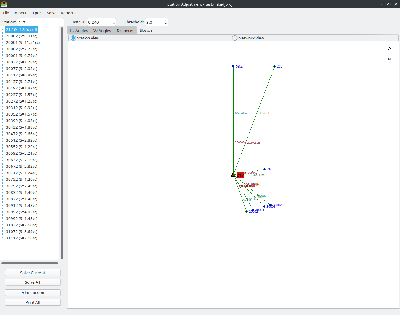
Sketch tab in Station View mode showing the selected station and its observed points.

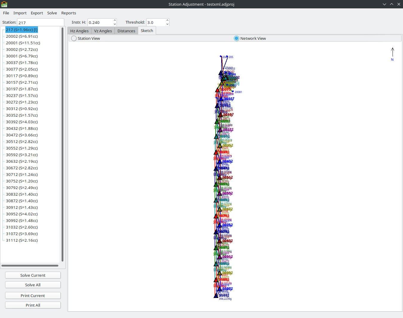
Sketch tab in Network View mode showing all stations and observation connections.

2.1.1.10. References

The mathematical methods implemented in the Station Adjustment module are based on classical surveying adjustment theory. For further study, the following references are recommended:

Rosikopoulos, D. — Topographic Networks and Computations (Topografika Diktya kai Ypologismoi). Comprehensive treatment of survey network adjustment, observation equations, least-squares methods, and statistical testing for geodetic and engineering survey networks.
Vlachos, D. — Topography, Volume 3 (Topografia, Tomos 3). Detailed coverage of instrument adjustment procedures, station observation methods (sets of angles, face I/II), collimation error correction, and practical field measurement techniques.
LandXML 1.2 Schema Specification — http://www.landxml.org/schema/LandXML-1.2/ — Standard schema for exchange of survey and civil engineering data.
Leica Geosystems — Leica Captivate Technical Reference Manual — Documentation of the LandXML export format used by Leica total stations, including the structure of <InstrumentSetup>, <ObservationGroup>, and <RawObservation> elements.
Leica Geosystems — GSI Online for Leica TPS — Official documentation of the GSI (GEO Serial Interface) data format, including Word Index tables, data block structure, and format variants (GSI8/GSI16).
Total Open Station — GSI Format Reference — https://totalopenstation.readthedocs.io/en/stable/input_formats/if_leica_gsi.html — Open-source documentation of the Leica GSI format with word index tables and examples.
MicroSurvey — STAR*NET Reference Manual — Documentation of the STAR*NET data file format for network adjustment, including direction sets (DB/DM/DE), observation records, and inline options.