2.1.2. Network Adjustment

2.1.2.1. Overview

The Network Adjustment module performs a rigorous least-squares adjustment of a survey network. Where the Station Adjustment module reduces the observations made at one instrument setup, the Network Adjustment module ties many stations together into a single geometric network and computes the most probable coordinates of every unknown point, together with full statistical quality indicators (standard deviations, error ellipses, residuals and blunder detection).

Typical inputs are terrestrial observations — horizontal angles, directions, azimuths/bearings, zenith angles, slope and horizontal distances, height differences — referenced to one or more control (fixed) points. The module solves a combined 3-D network (or a reduced 2-D / 1-D network) and reports adjusted coordinates and a complete error analysis.

Projects are stored in a single .adjproj file (an SQLite database), the same container used by Station Adjustment, so adjusted setups can be bridged directly into a network (see Bridge: pull adjusted stations).

Note

Internally all coordinates and distances are held in metres and all angles in gradians/gon (400 gon = full circle). The units you see and type (Meters / US Feet / International Feet, and GONS / DMS) are a presentation choice configured on the Settings tab; conversions happen only at the edges (grids, dialogs, reports and ASCII import/export).

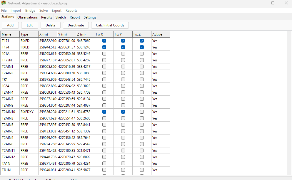
The Network Adjustment window: the tabbed workspace with the menu bar and the status line at the bottom. The window title shows the open project file name.

2.1.2.2. Getting Started

2.1.2.2.1. Opening the module

Open the module from the sidebar under Calculations > Network Adjustments. It opens as a separate window with a menu bar (File / Import / Bridge / Solve / Export / Reports) and a tabbed workspace.

2.1.2.2.2. Creating or opening a project

• File > New Project — choose a location and a file name (extension .adjproj). An empty SQLite project is created.

• File > Open Project — select an existing .adjproj file.

• File > Close Project — releases the project file.

Note

A project file is opened exclusively. Close the project (or the window) before opening the same file in the Station Adjustment module, otherwise you will get a “file is open” error. Closing the Network Adjustment window automatically closes the project.

The window title bar shows Network Adjustment - <filename> for the open project.

2.1.2.2.3. The workspace tabs

The workspace is organised into six tabs:

Tab	Purpose
Stations	Station list with coordinates, type (fixity) and instrument height; the Calc Initial Coords command.
Observations	All measurements (angles, distances, zeniths, …) with the Active flag for including/excluding each one.
Results	Adjusted coordinates and their standard deviations, shown after a successful solve.
Sketch	A scaled plan view of the network (stations + observation lines + error ellipses), with zoom and pan.
Report	The full text adjustment report.
Settings	Units, adjustment type, scale/projection, convergence and default instrument standard errors.

2.1.2.3. Concepts

2.1.2.3.1. Station types (fixity)

Every station has a type that tells the adjustment which of its coordinates are held fixed (control) and which are unknowns to be solved. The same vocabulary is used in the Stations grid, the Edit Station dialog and the .iqnet file:

Type	Meaning	Held fixed
FREE	Fully unknown point — solved in X, Y and Z	nothing
FIXED	Full control — coordinates held exactly	X, Y and Z
FIXEDXY	Horizontal control with unknown height	X and Y (Z is solved)
FIXEDZ	Benchmark / known height with unknown position	Z (X and Y are solved)

On the Stations grid the three check-box columns Fix X / Fix Y / Fix Z let you set the held components directly; the Type column shows the resulting classification. A network needs enough fixed control to define its datum (position, orientation and scale) — at minimum two fixed horizontal points (or a fixed point plus a fixed bearing), and at least one fixed height for a 3-D/1-D solve.

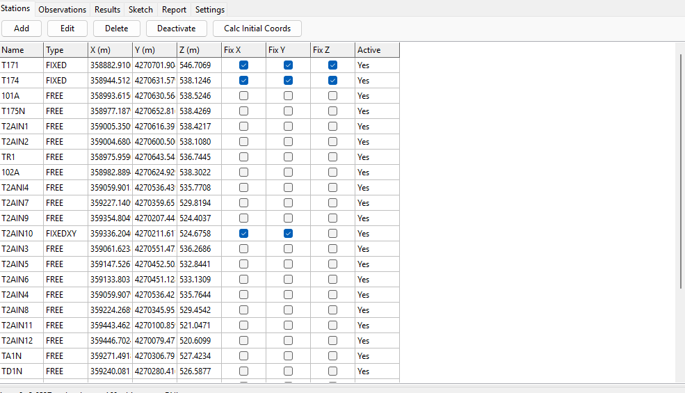
The Stations tab: the toolbar (Add / Edit / Delete / Deactivate / Calc Initial Coords) and the station grid with the Fix X / Fix Y / Fix Z check-boxes and the Type column.

2.1.2.3.2. Observation types

Type	Description
Angle	Horizontal angle measured at a station, from a backsight to a foresight (At-From-To).
Direction	Horizontal circle reading from a station to a target.
Azimuth	Absolute azimuth/bearing from one station to another.
Zenith	Vertical (zenith) angle, used for trigonometric heighting.
SlopeDistance	Measured slope distance between two stations.
HorizDistance	Measured horizontal distance.
HeightDiff	Levelled height difference (used by 1-D / leveling networks).
GPS baseline	Imported for reference only — not adjusted (the engine has no GPS vector model).

Each observation carries a standard error (its weight), an instrument height (HI) and target height (HT) where relevant, and an Active flag. De-activating an observation (uncheck Active) removes it from the solve without deleting it.

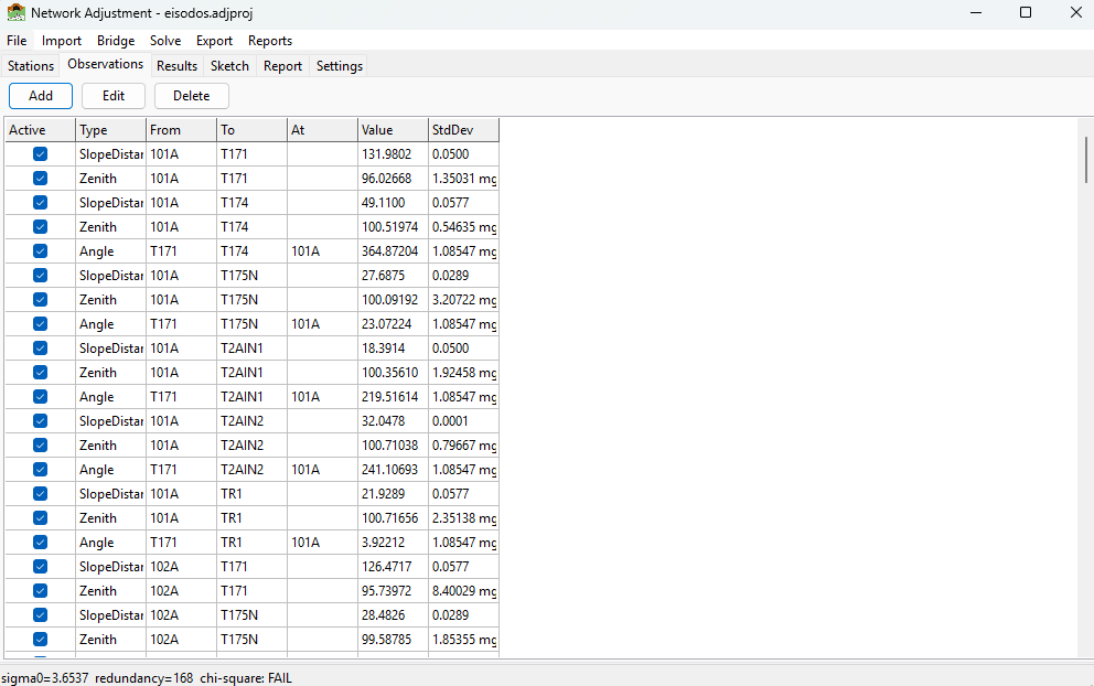
The Observations tab: each measurement with its type, stations, value, standard deviation, and the Active check-box.

2.1.2.3.3. Units and standard errors

Angular standard errors are entered in milligon (mgon) when the angular unit is GONS, or arc-seconds when it is DMS. Linear standard errors are in the current linear unit. The default instrument standard errors on the Settings tab are applied to any imported observation that does not carry its own value.

2.1.2.4. Settings

The Settings tab controls how the network is reduced and solved. Click Apply Settings to store changes in the project.

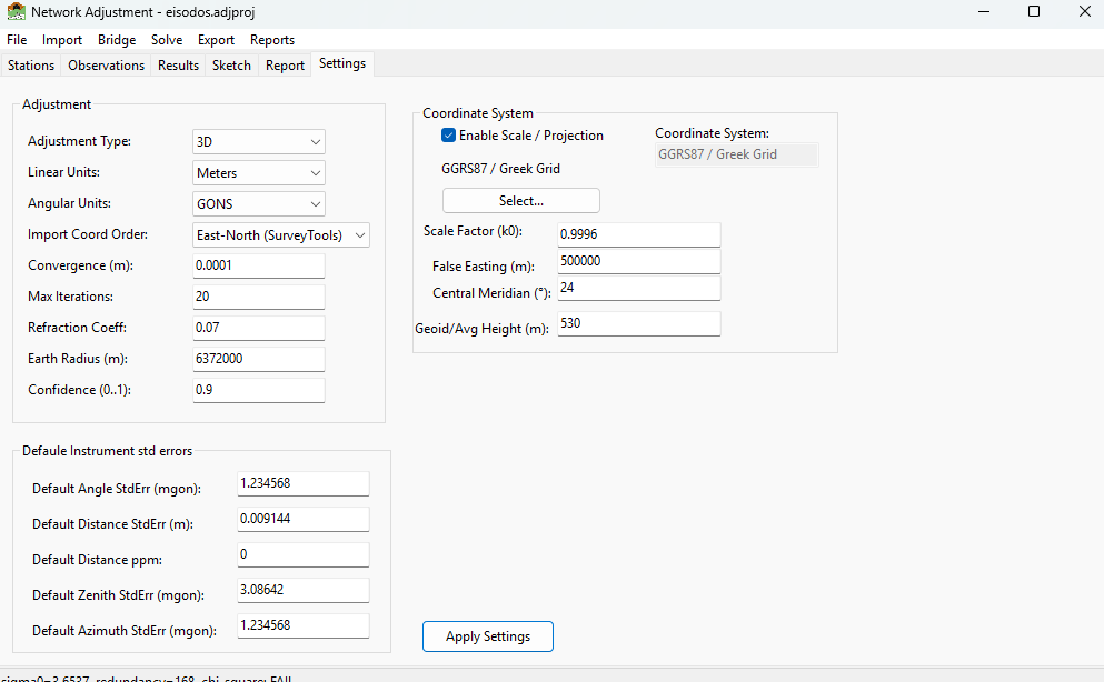
The Settings tab. Top group: units and solve controls. Middle group: scale/projection. Bottom group: default instrument standard errors.

Setting	Meaning
Adjustment Type	3D (X, Y, Z), 2D (horizontal only) or 1D (heights/levelling only).
Linear Units	Meters / US Feet / Intl Feet — display + ASCII I/O unit.
Angular Units	GONS or DMS — display + ASCII I/O unit.
Import Coord Order	Column order for .dat/.iqnet files that do not declare their own order: East-North (SurveyTools) or North-East (StarNet). See Coordinate order (East-North vs North-East).
Convergence (m)	Iteration stops when the largest coordinate correction falls below this value.
Max Iterations	Upper bound on least-squares iterations.
Refraction Coeff	Coefficient k of atmospheric refraction used in the curvature-and-refraction correction for trig heights.
Earth Radius (m)	Mean earth radius R used in the same correction and in grid reductions.
Confidence (0..1)	Confidence level for the reported error ellipses (e.g. 0.95 = 95 %).
Coordinate System	Read-only label, filled from the selected projection; printed on the report. See Coordinate order (East-North vs North-East).
Enable Scale / Projection	Turns on grid/projection reductions (k0, false easting, central meridian, geoid height). When off, observations are treated as plane/ground measurements.
Scale Factor (k0)	Central scale factor of the Transverse-Mercator grid.
False Easting (m)	Grid false easting.
Central Meridian	Longitude of the central meridian (degrees).
Geoid/Avg Height (m)	Average geoid/terrain height folded into the elevation (sea-level) reduction of distances.
Default …StdErr	Default instrument standard errors (angle, distance + ppm, zenith, azimuth) for observations without their own.

2.1.2.4.1. Choosing a projection

With Enable Scale / Projection ticked, click Select… to pick a coordinate system from the EPSG database (see the Appendix: EPSG Transformations). The chosen system fills the read-only Coordinate System field and the k0 / false easting / central meridian values; that name is what appears on the report. With scale disabled the Coordinate System field is cleared.

2.1.2.5. Building a network

You can build a network three ways: by importing a data file (Importing data), by bridging adjusted setups from Station Adjustment (Bridge: pull adjusted stations), or by entering stations and observations by hand.

2.1.2.5.1. Editing by hand

On the Stations tab use Add / Edit / Delete to manage points. The Edit Station dialog takes the name, X/Y/Z (in the current linear unit), the Type (FREE / FIXED / FIXEDXY / FIXEDZ) and the instrument height.

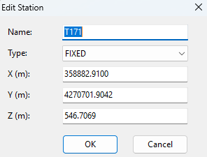
The Edit Station dialog.

On the Observations tab use Add / Edit / Delete. The Edit Observation dialog adapts to the chosen type: the At station is enabled only for Angle observations, and the Value / StdDev fields are formatted for linear or angular units automatically.

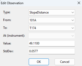
The Edit Observation dialog.

2.1.2.6. Importing data

2.1.2.6.1. STAR*NET .dat files

Import > STAR*NET (.dat)…

SurveyTools reads a broad subset of the STAR*NET .dat data format — a plain-text, line-oriented format widely used in survey adjustment. The importer is stateful: directives (lines beginning with .) set a parse context, and each data line is interpreted in that context.

Recognised directives include:

• .3D / .2D / .1D / .3REDUCE — adjustment dimension;

• .ORDER — coordinate column order (NE/EN) and angle order (AtFromTo/FromAtTo);

• .UNITS — linear and angular units for the values that follow;

• .DELTA, .SCALE, .REFRACTION, .INSTRUMENT, .SEPARATOR, .CURVE, .DATA ON/OFF, .INCLUDE and others.

Recognised data codes include:

Code	Meaning
C CH	Coordinate station (full X/Y/Z; CH = ellipsoid height).
E EH	Elevation-only station (levelling form).
P PH	Latitude/longitude station, forward-projected to grid E/N.
A	Horizontal angle (At-From-To).
B	Bearing / azimuth (quadrant bearings supported).
D M	Distance (M = combined angle/distance/zenith measurement).
V	Zenith angle.
S Z	Rawdata-dialect slope distance / zenith.
L	Levelling height difference (solves as a 1-D network).
TB T TE	Traverse macros (backsight / course / end) expanded to angles and distances.
G1 G2 G3	GPS vectors — imported for display only, not adjusted.

Fixity is taken from the per-coordinate flags after the coordinates (! = fixed, * = free). A station with no flags is treated as an approximate / free point (control points carry ! ! !), except in the rawdata (S/Z) dialect where a bare C is control.

After import, a summary dialog lists how many stations and observations were read, plus any warnings (skipped lines, GPS notices, weighted-coordinate notes).

example_network.dat - a small STAR*NET-style file

# SurveyTools / STAR*NET-style data file (.dat) - example
#
# STAR*NET(R) is a registered trademark of MicroSurvey Software Inc.
# SurveyTools reads a broad subset of the STAR*NET .dat format; it is an
# independent implementation and is not affiliated with or endorsed by
# MicroSurvey Software Inc.
#
# Directives configure the parse context; data lines are interpreted in context.

.3D                       # 3-D adjustment (also .2D, .1D, .3REDUCE)
.ORDER AtFromTo           # angle triples are At-From-To
.UNITS METERS GONS        # linear = metres, angular = gradians (gon)

# --- Coordinates (C = full X/Y/Z, '! ! !' = fixed; no flags = approximate/free)
C ST1 358882.9100 4270701.9042 546.7069 ! ! !
C ST2 358944.5123 4270631.5791 538.1246 ! ! !
C N1  358993.6156 4270630.5644 538.5246
C N2  359005.3509 4270616.3975 538.4217

# --- Observations
# A = angle (At-From-To), D = slope distance, V = zenith; trailing value = std-err
A ST1-ST2-N1 50.1234 1.0
D ST1-N1 149.5890 0.005
V ST1-N1 98.7654 3.0

A ST1-N1-N2 42.0000 1.0
D ST1-N2 131.9760 0.005
V ST1-N2 103.9230 3.0

2.1.2.6.2. Coordinate order (East-North vs North-East)

STAR*NET files default to North-East column order, while SurveyTools’ own files use East-North. If a file does not contain an explicit .ORDER directive, the Import Coord Order setting decides how its first two coordinate columns are read. Set it to North-East (StarNet) before importing a native STAR*NET file, or leave it at the default East-North (SurveyTools) for SurveyTools/.iqnet files. An in-file .ORDER directive always wins.

2.1.2.6.3. Editable ASCII project files (.iqnet)

Import > ASCII Project (.iqnet)… and Export > ASCII Project (.iqnet)…

The .iqnet format is a single, human-editable text file that captures a whole project — settings, initial coordinates and measurements — so you can edit a network quickly in any text editor and read it back, or move it to a new project. It has three sections in fixed order, [SETTINGS], [STATIONS] and [OBSERVATIONS]; # starts a comment. Values are written in the units declared in [SETTINGS].

Important

Import is “Replace”. Importing an .iqnet file clears the open project’s settings, stations and observations and loads them entirely from the file. The file is parsed completely before anything is changed, so a malformed file never leaves a half-loaded project. Unknown keys or observation types are reported as warnings and skipped.

Station fixity uses the same FREE / FIXED / FIXEDXY / FIXEDZ labels as the rest of the module. Observation rows are tagged ANG, DIR, AZ, ZEN (angular) and DIST, HDIST, DH (linear); the At column is used only by ANG. GPS baselines are written as comments (informational).

example_network.iqnet - a complete project file

# SurveyTools Network Adjustment - example project file (.iqnet)
# Format v1
#
# Three sections in fixed order: [SETTINGS], [STATIONS], [OBSERVATIONS].
# '#' starts a comment (to end of line). Blank lines are ignored.
# Linear values are in LinearUnits, angles in AngularUnits (see [SETTINGS]).

[SETTINGS]
LinearUnits         = Meters         # Meters | FeetUS | FeetInt
AngularUnits        = GONS           # GONS | DMS
CoordOrder          = EN             # EN | NE  (X/Y column order below)
AdjustmentType      = 3D             # 1D | 2D | 3D
ScaleEnabled        = 1              # 0 | 1  (apply grid/projection reductions)
CoordinateSystem    = HGRS87 / Greek Grid (TM)
ProjK0              = 0.9996
ProjFalseEasting    = 500000
ProjCentralMeridian = 24
GeoidHeight         = 530
EarthRadius         = 6372000
RefractionCoeff     = 0.13
Convergence         = 0.0001
MaxIterations       = 50
Confidence          = 0.95
OutlierThreshold    = 3.0
StdAngle_mgon       = 1.0
StdDist_m           = 0.003
StdDist_ppm         = 2.0
StdZenith_mgon      = 3.0
StdAzimuth_mgon     = 1.0

[STATIONS]
# Name        X(E)          Y(N)           Z        Type      HI
# Type: FREE | FIXED | FIXEDXY (X,Y held) | FIXEDZ (Z held)
ST1      358882.9100   4270701.9042    546.7069    FIXED     1.500
ST2      358944.5123   4270631.5791    538.1246    FIXED     1.500
N1       358993.6156   4270630.5644    538.5246    FREE      0.000
N2       359005.3509   4270616.3975    538.4217    FREE      0.000

[OBSERVATIONS]
# Type  At     From    To       Value      StdDev    HI     HT     Active
# Tags: ANG DIR AZ ZEN (angular) | DIST HDIST DH (linear). At only for ANG.
# Angular StdDev in mgon (GONS) / arcsec (DMS); linear StdDev in LinearUnits.
ANG     ST1    ST2     N1       50.1234    1.0       1.50   1.60   1
DIST    -      ST1     N1      149.5890    0.005     1.50   1.60   1
ZEN     -      ST1     N1       98.7654    3.0       1.50   1.60   1
ANG     ST1    N1      N2       42.0000    1.0       1.50   1.60   1
DIST    -      ST1     N2      131.9760    0.005     1.50   1.60   1
ZEN     -      ST1     N2      103.9230    3.0       1.50   1.60   1
# GPS baselines (G1/G2/G3 in StarNet) are exported here only as comments;
# the engine has no GPS solver, so they are informational and not adjusted.

2.1.2.6.3.1. Template

Export > ASCII Template (.iqnet)… writes a documented, empty template — all section headers, default settings, and commented example rows for every station type and observation type — so you can author a project from scratch.

2.1.2.6.4. Excel workbooks (.xlsx)

Import > Excel Workbook (.xlsx)… and Export > Excel Workbook (.xlsx)…

The Excel workbook is the spreadsheet twin of the .iqnet file: a two-sheet workbook (Stations and Observations) holding the station list (name, X/Y/Z, fixity, instrument height) and every measurement, written in the project’s current display units (the units are named in a header cell, so the file is self-describing). Use it to prepare or edit a network in Excel and read it back.

• Import is “Replace” — like .iqnet, importing clears the stations and observations and loads them from the file. Project settings are not overwritten. Unknown observation types and malformed rows are reported as warnings and skipped.

• Export > Excel Template (.xlsx)… writes an empty workbook with the headers plus an Instructions sheet documenting every column and the accepted type labels, so you can author a network from scratch in Excel.

2.1.2.6.5. Netsist projects (.ndb / DATA IN .xlsx)

Import > Netsist (.ndb, .xlsx)…

SurveyTools reads networks from the Netsist adjustment package in two forms, selected automatically from the file you pick:

• Netsist project database (.ndb) — the full project: stations with coordinates and control status (Netsist KNOWN points become FIXED), total-station observations with their direction sets and per-observation active flags, GNSS baselines, spirit-levelling lines and azimuths. Both the geodetic and the levelling database layouts are recognised.

• DATA IN measurement workbook (.xlsx) — Netsist’s measurement-entry template (sheets Stations, TotalStation(ddz), TotalStation(adz), GNSS Baseline, Spirit Levelling, Azimuth; the levelling variant of the template is also recognised). The template carries no fixity, so all stations import as FREE — set the control points afterwards on the Stations tab.

Like the other project-file imports, a Netsist import replaces the current stations and observations, and finishes with a log dialog listing what was read and any warnings.

Direction sets. Netsist groups direction readings into numbered sets, and each (station, set) pair gets its own orientation unknown in the solve. SurveyTools imports the set numbers and solves them the same way, so a network measured in several rounds adjusts exactly as it does in Netsist.

Spirit levelling weight. Netsist stores each levelling line’s length in km and weights it from a levelling accuracy a (the standard error is a·sqrt(L)). When a Netsist settings file (.nex) sits next to the imported file, the accuracy is taken from it automatically; otherwise you are asked for it (default 0.010 m/sqrt(km)).

Export > Netsist DATA IN (.xlsx)…

Writes the current stations and active observations back to the DATA IN template so the network can be opened in Netsist. A pure levelling project (only height differences) is written in the template’s levelling variant; anything else uses the full 3-D template. If the project contains height differences you are asked for the levelling accuracy again, so each observation’s standard error can be converted back to a line length (L = (σ/a)²).

Note

The DATA IN template stores measurements only: station fixity, inactive observations and the adjustment settings are not part of the format. Inactive observations are skipped (the export log says how many), and a re-imported file has all stations FREE.

2.1.2.7. Initial (provisional) coordinates

A least-squares network solve is iterative and needs approximate starting coordinates for every unknown point. If you only have control points plus observations, use Stations tab > Calc Initial Coords to compute them automatically. The engine propagates outward from the fixed/known points, repeatedly applying these geometric methods until no further point can be placed:

• Polar — a known station, an azimuth to the unknown and a distance.

• Traverse — a known occupied station, a known backsight, the turned angle to the unknown and the distance (bearing = backsight azimuth + angle).

• Backsight-angle reversal — when the unknown is observed only as the backsight of an angle at a known station (plus one distance), the direction to it is recovered from a known foresight.

• Intersection — two or more directions to the unknown from known stations (no distance needed).

• Trilateration — two or more distances from known stations.

• Resection — the unknown is the occupied station of three or more angles to known targets.

• Heights — Z is propagated separately from height differences, or from zenith + slope distance (with curvature-and-refraction correction).

A summary reports how many points were computed and lists any that could not be placed (for example a point with too few observations, or one reachable only through GPS baselines).

Note

These are approximate coordinates intended only to seed the adjustment. The final, rigorous coordinates come from the solve. Computed positions are also drawn on the Sketch tab so you can sanity-check the geometry before solving.

2.1.2.8. The least-squares adjustment

Run the adjustment from Solve > Solve (or Solve > Solve (Robust) for an outlier-resistant pass). Solve > Check Data… validates the network first (see Checking the data).

2.1.2.8.1. What the solve computes

The module forms one observation equation per measurement, linearises it about the approximate coordinates, and solves the resulting normal equations by weighted least squares (a Gauss-Newton iteration). Each observation is weighted by the inverse square of its standard error, so precise measurements pull harder than rough ones. The corrections to the unknown coordinates are applied, and the process repeats until the largest correction is below Convergence (or Max Iterations is reached).

2.1.2.8.2. Reductions applied before the solve

When Enable Scale / Projection is on, raw ground measurements are reduced to the grid so they are geometrically consistent with projected (E, N) coordinates:

• Elevation (sea-level) reduction — distances are scaled from the average station/terrain height (and the Geoid/Avg Height) down to the ellipsoid, using the Earth Radius.

• Grid scale factor — the Transverse-Mercator scale (from k0 and the distance from the Central Meridian) is applied so distances match grid distances.

• Curvature and refraction — trigonometric height differences from zenith angles are corrected with the Refraction Coeff and Earth Radius.

With scale disabled, measurements are adjusted as plane/ground values with no grid reduction.

2.1.2.8.3. Dimension (1-D / 2-D / 3-D)

• 3-D solves X, Y and Z together (angles, distances and zeniths).

• 2-D reduces slope distances to horizontal and solves X, Y only.

• 1-D solves heights only from height differences / levelling — useful for pure levelling networks (an imported levelling .dat switches to this mode automatically).

2.1.2.9. Results and quality

2.1.2.9.1. Adjusted coordinates

After a successful solve the Results tab lists each station’s adjusted X, Y, Z and the coordinate standard deviations σx, σy, σz.

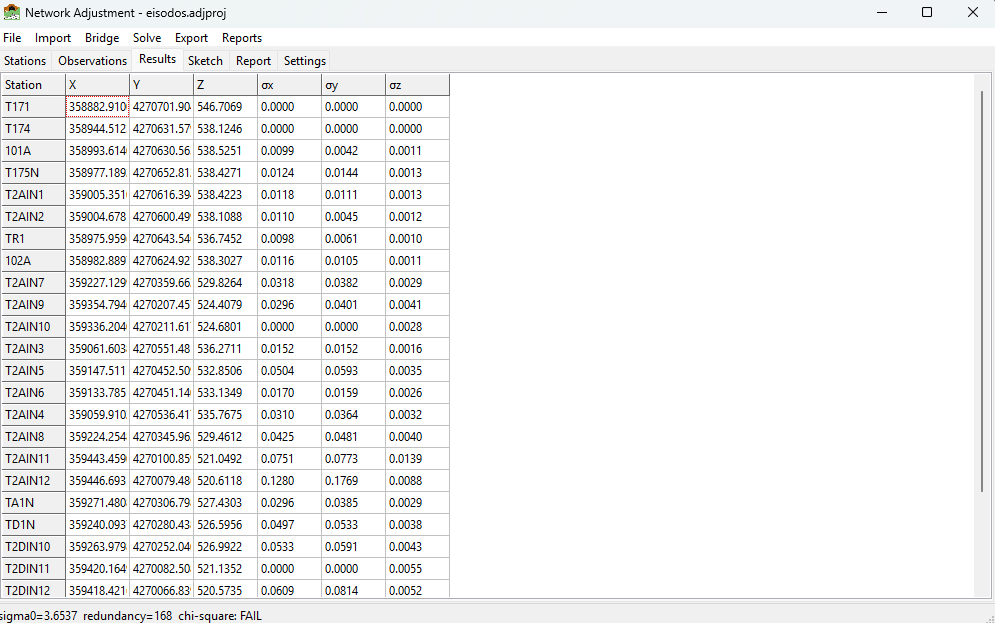
The Results tab after a successful adjustment.

2.1.2.9.2. Statistics in the report

The Report tab (and the exported reports) contain the full error analysis:

• A-posteriori reference factor (σ₀, the standard error of unit weight) — a value near 1.0 indicates the observation standard errors are realistic. Much larger than 1 suggests over-optimistic weights or blunders; much smaller suggests pessimistic weights.

• Adjusted observations and residuals — the correction applied to each observation; large standardised residuals point to suspect measurements.

• Coordinate standard deviations for every adjusted point.

• Error ellipses — the semi-major/semi-minor axes and orientation of each point’s confidence ellipse, at the configured Confidence level, also drawn on the Sketch.

• Adjusted azimuths and horizontal distances between connected points, with the ground distance printed beside the grid distance.

• Error factors by observation type — the a-priori standardised residuals of each group over the group’s summed redundancy numbers, so a type whose factor stands out from the Total row is the one whose standard errors are wrong. Relative confidence columns (azimuth, distance) use the 2-D 95 % factor, the same as the error ellipses.

• Chi-square test — when the adjustment fails it, the error-propagation tables carry the note Adjustment Failed the Chi-Square Test / Scaled by Total Error Factor, so the inflated standard deviations are not read as a-priori precision.

Zenith, slope-distance and horizontal-distance observation equations are evaluated in ground space: they are ground measurements, so the grid coordinate separation is un-reduced by the combined grid factor before the comparison. Residuals therefore come out in the same units as the observations’ standard errors.

2.1.2.9.3. Robust solve and outliers

Solve (Robust) runs an iteratively re-weighted adjustment (Danish method): observations with large residuals are progressively down-weighted so a single blunder does not distort the whole network. The Outlier Threshold (in the Settings) controls how aggressively suspect observations are flagged. Use it to locate a blunder, fix or de-activate the offending observation, then re-solve normally.

2.1.2.9.4. Checking the data

Solve > Check Data… reports problems that would prevent or distort a solve — for example observations that reference a non-existent station (orphan observations), active stations not referenced by any observation, or an insufficiently constrained datum. Errors block the solve; warnings do not.

2.1.2.10. The Sketch

The Sketch tab draws a scaled plan view: stations at their current coordinates (adjusted if available, otherwise initial), the observation lines that connect them, and — after a solve — the error ellipses. Use Zoom Extents, + / -, the mouse wheel to zoom, and drag to pan. The sketch is a quick way to confirm the network geometry and spot a mis-keyed coordinate.

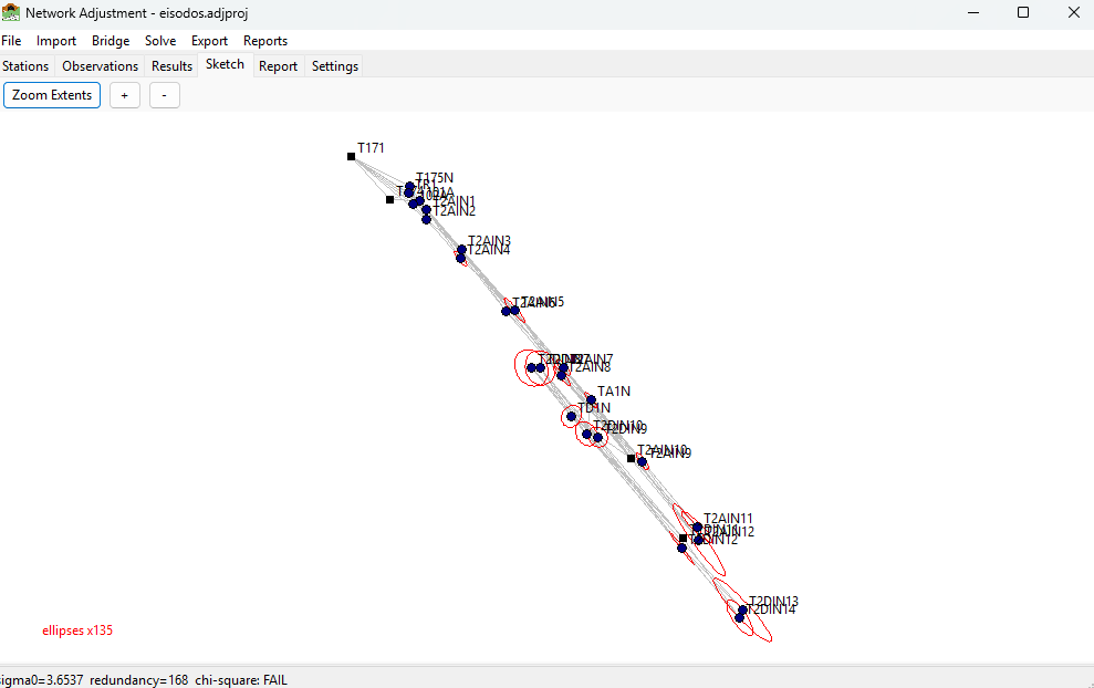
The Sketch tab showing stations, observation lines and error ellipses.

2.1.2.11. Bridge: pull adjusted stations

Bridge > Pull Adjusted Stations imports the results of the Station Adjustment module (held in the same .adjproj file) into the network: for every station that has saved station-adjustment results, the adjusted directions, zeniths and distances to its targets are converted into network observations (with their standard errors carried across), ready to be solved as a network. Existing observations from a previous pull are replaced, so the command is safe to repeat.

2.1.2.12. Reports and export

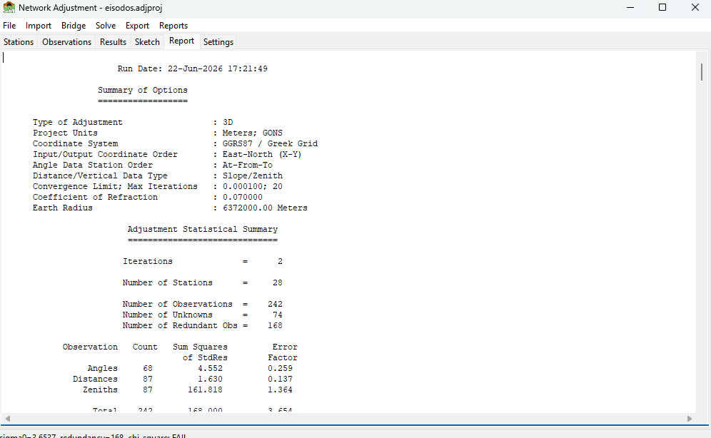
The Report tab showing the full text adjustment report.

• Reports > Full Text Report… — writes the complete adjustment report to a .txt file, honouring the chosen units. It opens with a STAR*NET-style Summary of Files Used and Option Settings — project name, title, description, folder and file, client, location, surveyor, created and modified dates, then every setting that went into the solve (adjustment type, units, coordinate system and projection preset, grid reduction and its k0 / false easting / central meridian, geoid height, earth radius, refraction coefficient, coordinate orders, convergence limit and iteration cap, confidence region, outlier threshold, angle decimals), the default instrument standard errors and, when the network carries baselines, the GNSS settings — so a run can be reproduced from the report alone. Then follow the input observations, statistics, adjusted coordinates, residuals and error ellipses.

• Reports > Export PDF… — a formatted PDF report. Use Reports > Company Info… to set the firm/surveyor details, logo and accent colour printed on it.

• Export > Coordinate List (CSV)… — adjusted coordinates as CSV.

• Export > STAR*NET (.dat)… — the network as a STAR*NET-style data file.

• Export > ASCII Project (.iqnet)… / ASCII Template (.iqnet)… — see Editable ASCII project files (.iqnet).

• Export > Excel Workbook (.xlsx)… / Excel Template (.xlsx)… — the stations + observations workbook, see Excel workbooks (.xlsx).

• Export > Netsist DATA IN (.xlsx)… — the network as a Netsist DATA IN measurement workbook, see Netsist projects (.ndb / DATA IN .xlsx).

2.1.2.13. Typical workflow

1. File > New Project (or open an existing one).

2. On Settings, set the units, adjustment type, and — if working on a grid — enable Scale / Projection and pick the coordinate system; set the default instrument standard errors. Apply Settings.

3. Bring in data: Import a .dat/.iqnet file, Bridge from Station Adjustment, or add stations/observations by hand. Set the control points’ fixity.

4. If the unknowns have no coordinates yet, Stations > Calc Initial Coords.

5. Solve > Check Data…, then Solve > Solve.

6. Review the Results, Report and Sketch. If σ₀ is large or a residual stands out, use Solve (Robust) to find the blunder, correct or de-activate it, and re-solve.

7. Export the coordinates / report, or Export ASCII Project to archive an editable copy.

2.1.2.14. Trademarks

STAR*NET^® is a registered trademark of MicroSurvey Software Inc. SurveyTools provides an independent implementation that reads and writes a subset of the STAR*NET data file format for interoperability; it is not affiliated with, endorsed by, or sponsored by MicroSurvey Software Inc. Netsist is a product of its respective owner; SurveyTools reads and writes Netsist file formats for interoperability only and is not affiliated with or endorsed by its publisher. All other trademarks are the property of their respective owners.