2.2.1. Special Monitoring Adjustment

2.2.1.1. Overview

The Special Monitoring Adjustment tool processes multiple measurement sets recorded at a single monitoring station — the typical deformation monitoring workflow where every target point is observed with many repeated readings per telescope face, in several sets (rounds of the horizon).

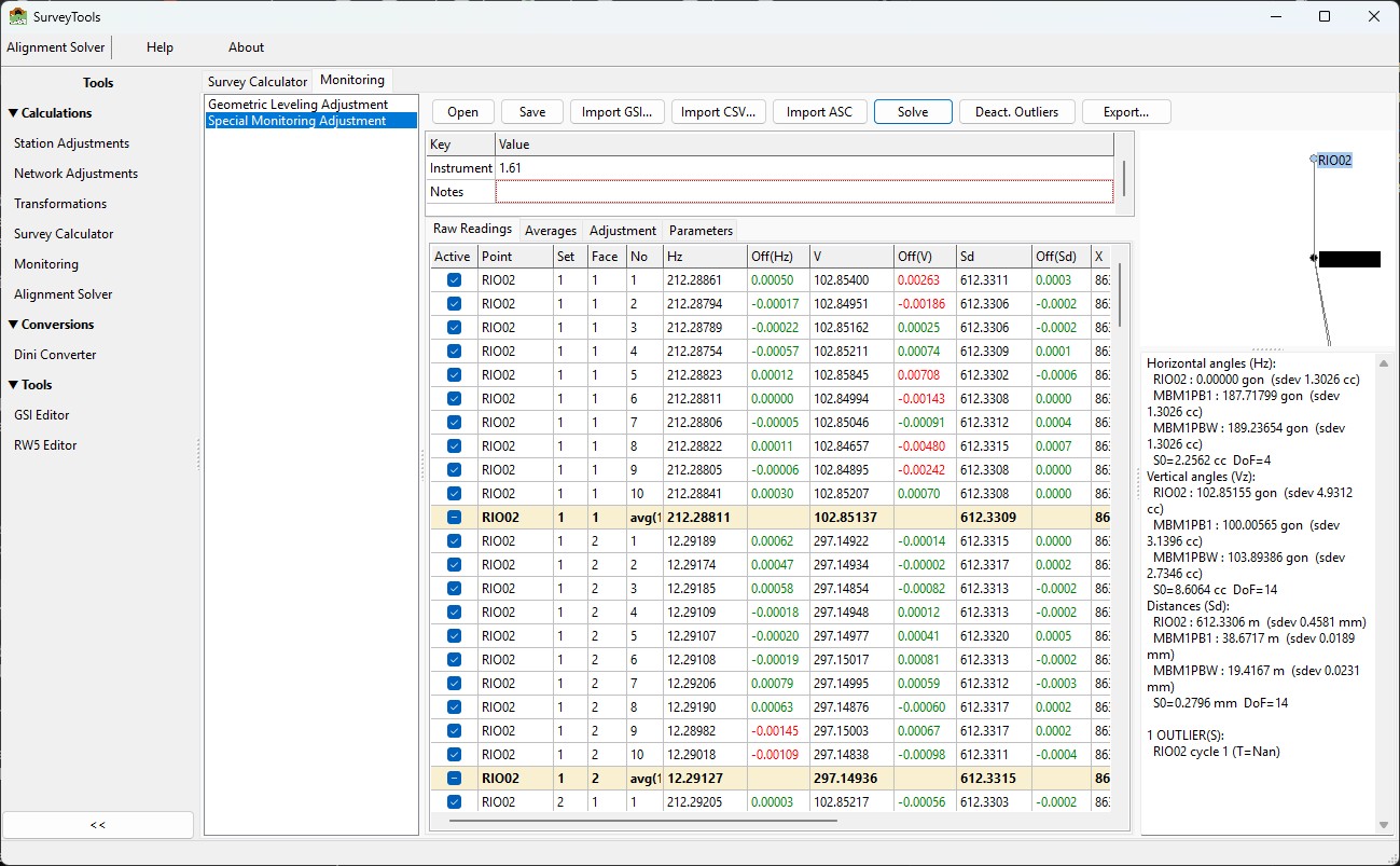
../../_images/monitoring_station_1.jpg — The Special Monitoring Adjustment tool: the Raw Readings tab with the per-reading offsets and set averages, and the station results (Hz/Vz/Sd averages, standard deviations and flagged outliers) in the panel on the right.

The tool works in three stages, each with its own tab:

Raw Readings — every single pointing of the instrument, grouped by point, set and face, with the deviation (offset) of each reading from its group average. Individual readings can be deactivated with a checkbox; everything downstream recalculates immediately.
Averages — per set: the Face I and Face II averages, their standard deviations and the face-combined value for Hz, V and Sd (plus the mean X/Y/Z coordinates); per point: the overall average over all sets and its M.Sdev (the standard deviation of the set averages).
Adjustment — the per-set averages are adjusted with the same least-squares station adjustment used by the Station Adjustment module (see Station Adjustment): adjusted directions / zenith angles / distances per point, per-observation residuals with the R and T outlier statistics, and the solve statistics.

All angles are in gradians (400 grads per full circle). Angle residuals are expressed in centesimal seconds (cc), distance residuals in millimeters (mm). Coordinates and distances are in meters.

2.2.1.2. Opening the Tool

Open it from the sidebar under Calculations > Monitoring and select Special Monitoring Adjustment from the calculation list.

The window has a toolbar (Open / Save / Import GSI / Import CSV / Import ASC / Solve / Deact. Outliers / Export), a station info panel (station name, instrument height, notes), the four data tabs, and on the right a schematic sketch plus a text summary of the last solve.

2.2.1.3. Concepts

Term	Meaning
Reading	One single pointing of the instrument: Hz, V, Sd (+ X, Y, Z as computed by the instrument). Typically ~10 readings are recorded per point, per face, per set.
Face	Telescope position. Face I readings have a zenith angle below 200 gon; Face II readings are the “plunged” pointings (Hz ≈ Face I + 200 gon, V ≈ 400 − Face I).
Set	One full round of the horizon: all points in Face I, then all points in Face II (usually in reverse order). Sets are repeated — 3 sets is common for monitoring.
Face average	Mean of the active readings of one point/set/face group (bold rows in the Raw Readings tab).
Set average	The Face I and Face II averages of one point in one set, plus the face-combined value (Hz: `(I + (II ∓ 200)) / 2`, V: `(I + (400 − II)) / 2`, Sd: plain mean).
Point average / M.Sdev	Mean of a point’s set averages over all sets, and the standard deviation of those set averages.
Offset	Deviation of one reading from its face average (wrap-aware for angles). Offsets are colour-coded against the alarm levels of the Parameters tab.

2.2.1.4. Importing Data

The tool reads three file formats. The ASC and GSI formats carry raw repeated readings and feed the full three-stage pipeline; the CSV format carries already-averaged face pairs and goes directly to the adjustment.

Sets and faces are never stored explicitly in the raw files — the importer detects them automatically:

Face: a reading with zenith angle V < 200 gon is Face I, otherwise Face II.
Set: readings arrive in blocks per point and face. Every time a point/face combination re-appears after a gap, a new set begins (the N-th block of a point/face = set N). The usual acquisition order — Face I forward through the points, Face II backward — is handled automatically.

2.2.1.4.1. Import ASC (raw readings)

Toolbar > Import ASC

One line per reading, comma-separated, 15 fields:

Point\NN,Hz,V,Sd,IH,RH,ppm,mm,month,day,hour,minute,X,Y,Z

MBM1PB4.asc (first lines)

RIO02\01,212.28861,102.85400,612.3311,1.6100,0.1950,21, 0,7, 26, 18, 36,863.2925,1057.9647,2.2976
RIO02\02,212.28794,102.84951,612.3306,1.6100,0.1950,21, 0,7, 26, 18, 36,863.2986,1057.9620,2.3407
RIO02\03,212.28789,102.85162,612.3306,1.6100,0.1950,21, 0,7, 26, 18, 36,863.2992,1057.9628,2.3205

Field	Description
`Point\NN`	Target point name and running reading number within the block (e.g. `RIO02\01` … `RIO02\10`).
`Hz`, `V`	Horizontal direction and zenith angle in gon.
`Sd`	Slope distance in meters.
`IH`, `RH`	Instrument height and reflector (target) height in meters.
`ppm`, `mm`	Atmospheric ppm correction and prism constant.
`month day hour minute`	Acquisition time (the format carries no year).
`X`, `Y`, `Z`	Coordinates of the target as computed by the instrument.

Notes:

An optional leading record index followed by a TAB (123<TAB>...) is accepted and stripped.
The station name defaults from the file name; the instrument height is taken from the IH column (a warning is shown if it is not constant).
A malformed line aborts the import with a message naming the line number.

2.2.1.4.2. Import GSI (raw readings or classic)

Toolbar > Import GSI

Leica GSI8/GSI16 files are auto-detected:

If the point names carry the Point\NN multiple-reading convention (e.g. RIO02\01), the file is treated exactly like an ASC file — every line is one raw reading and the full pipeline is used. Word indices read: 11 (point), 21 (Hz), 22 (V), 31 (Sd), 87/88 (target/instrument height), 51 (ppm/prism constant), 19 (date/time), 81/82/83 (X/Y/Z).

MBM1PB4.GSI (first line, GSI16)

*112266+00000000RIO02\01 21.322+0000000021228861 22.322+0000000010285400 31..06+0000000006123311 88..16+0000000000016100 87..16+0000000000001950 51..1.+000000000021+000 19....+0000000007261836 81..06+0000000008632925 82..06+0000000010579647 83..06+0000000000022976

If the point names are plain (a classic station-adjustment GSI file), the observations are imported as already-averaged face pairs — the Raw Readings and Averages tabs stay empty and only the adjustment runs.

2.2.1.4.3. Import CSV (averaged observations)

Toolbar > Import CSV

One already-averaged observation per line, no header:

PointName,Cycle,ObsType,FaceLeft,FaceRight,TargetHeight

sample_observations.csv (first lines)

CASTLE02,1,HZ,158.09718,358.09570,0.236
CASTLE02,1,VZ,102.86571,297.13715,0.236
CASTLE02,1,SD,417.8766,417.8764,0.236

Cycle is the set number (1-based).
ObsType is HZ, VZ or SD (case-insensitive) — each measurement type is its own line.
FaceLeft / FaceRight are the Face I / Face II values; leave a field blank for a single-face observation.
TargetHeight is optional (defaults to 0).

Warning

Do not open a raw .asc file with Import CSV — the two layouts are different (the CSV importer expects the observation type in the third field). The tool detects this mistake and points you to Import ASC.

2.2.1.5. The Tabs

2.2.1.5.1. Raw Readings

All readings grouped by point — all sets of a point together, ordered point > set > face > reading number — with a bold face-average row closing every group.

Column	Content
`Active`	Checkbox. Untick to deactivate a reading: it is excluded from all averages and the whole chain (averages, derived observations, next solve) recalculates immediately. Deactivated readings show no offsets.
`Hz, V, Sd, X, Y, Z`	The raw values of the pointing.
`Off(Hz) … Off(Z)`	Offset of the reading from its face average. Green when the absolute offset is at or below the alarm level, red when above it (see Parameters).
`avg(n)` rows	Face average over the n active readings of the group.

2.2.1.5.2. Averages

A selector switches between Horizontal (Hz), Vertical (V), Distance (Sd) and Coordinates (XYZ):

Hz/V/Sd views: one row per point per set with the Face I and Face II averages, their standard deviations and the face-combined Average; a bold avg(n) summary row per point holds the overall average and the M.Sdev (standard deviation of the set averages — the key repeatability indicator between sets).
XYZ view: the mean coordinates per set and the overall mean per point.

2.2.1.5.3. Adjustment

Filled after Solve (the tool switches to this tab automatically). A selector switches between Hz, Vz and Sd. For the selected type:

Adjusted values: point, adjusted direction / zenith angle / distance, and its standard deviation (cc for angles, mm for distances).
Observations: one row per point per set with the Face I/II input values, the combined average, the reduced direction (Hz only), the residuals v / v1 / v2, the standardized residual R, the studentized statistic T and an outlier flag (*, drawn in red).
The statistics line: a-posteriori S0, degrees of freedom, and the point / set / observation counts.

The mathematics are identical to the Station Adjustment module — the per-set face-combined averages enter the same least-squares round-of-horizon solution. See Station Adjustment for the algorithm and the meaning of the statistics.

2.2.1.5.4. Parameters

Alarm levels for the offset colouring of the Raw Readings tab:

Alarm	Default	Applies to
Angles (gon)	0.001	Off(Hz), Off(V)
Distance (m)	0.001	Off(Sd)
Coordinates (m)	0.001	Off(X), Off(Y), Off(Z)

Offsets above an alarm level render red; offsets at or below it render green. The levels are saved with the project.

2.2.1.6. Solving and Outliers

Solve recomputes the averages from the active raw readings, feeds the per-set averages into the station adjustment, and shows the results in the Adjustment tab, the summary memo and the schematic sketch.

Deact. Outliers deactivates all observations flagged as outliers by the last solve (per point and set) and re-solves. Use it after inspecting the T statistics in the Adjustment tab.

Note

Outlier deactivation works at the set average level (a whole point/set observation). To discard a single bad reading instead, untick its Active checkbox in the Raw Readings tab — that is usually the better first step.

2.2.1.7. Project Files

Save stores the whole campaign in a .monsta project file (XML): station info, alarm levels, all raw readings with their Active flags, and the derived observations. Open restores it and recomputes the averages. Projects written by older versions of the tool (format version 1, without raw readings) still load.

2.2.1.8. Exporting

Export… (after a solve) offers:

Excel workbook (XLSX) — three sheets mirroring the tabs: Raw Readings (all readings with offsets and face-average rows), Averages (per-set values, per-point average(n) and M.Sdev rows, X/Y/Z) and Adjustment (the three solved sections with residuals and statistics).
PDF report — an A4 report with the station info, point averages, set averages and the three adjustment sections (outlier rows printed red).

2.2.1.9. Sample Files

Use these files to try the complete workflow (3 points, 3 sets, 2 faces, 10 readings each — the ASC and GSI files contain the same campaign):

MBM1PB4.asc — raw readings, ASC format
MBM1PB4.GSI — raw readings, GSI16 format
sample_observations.csv — averaged observations, CSV format

Quick walk-through:

Import ASC (or Import GSI) and pick MBM1PB4.asc.
The Raw Readings tab shows 180 readings grouped under RIO02, MBM1PB1 and MBM1PBW with green/red offsets; check e.g. RIO02 set 1 face 1: average Hz 212.28811, V 102.85137, Sd 612.3309.
Open the Averages tab and compare the set averages and the M.Sdev of each point; switch the selector to see V, Sd and XYZ.
Untick a reading with a red offset and watch the averages update.
Solve — the Adjustment tab opens with the adjusted directions, residuals and statistics for Hz, Vz and Sd.
Export… the workbook and the PDF report.

2.2.1.10. Troubleshooting

Symptom	Cause / solution
Raw Readings and Averages tabs are empty after an import	The file contained no repeated readings: classic GSI files and CSV files carry averaged observations only. Use an ASC/GSI file with the `Point\NN` convention for the full pipeline.
“expected 15 comma-separated fields” on Import ASC	The line does not match the ASC layout — check for missing fields or a different export format.
“This looks like a raw multiple-readings file…” on Import CSV	You picked an `.asc` file in the CSV dialog; use Import ASC.
“Inconsistent instrument height in file”	The IH column changes mid-file; the first value is used. Verify the field data.
“Run Solve first” when exporting	The exports include the adjustment results — solve before exporting.